‘Analysis and Opinion’
The Data Dichotomy
Wednesday, December 14th, 2016
A post about services and data, published on the Confluent site.

https://www.confluent.io/blog/data-dichotomy-rethinking-the-way-we-treat-data-and-services/
The Benefits of “In-Memory” Data are Often Overstated
Sunday, January 3rd, 2016
There is an intuition we all share that memory is king. It’s fast, sexy and blows the socks off old school spinning disks or even new school SSDs. At it’s heart this is of course true. But when it comes to in-memory data technologies, alas it’s a lie. At least on balance.
The simple truth is this. The benefit of an in memory “database” (be it a db, distributed cache, data grid or something else) is two fold.
(1) It doesn’t have to use a data-structure that is optimised for disk. What that really means is you don’t need to read in pages like a database does, and you don’t have to serialise/deserialise between the database and your program. You just use whatever you domain model is in memory.
(2) You can load data into an in-memory database faster. The fastest disk backed databases top out bulk loads at around 100MB/s (~GbE network).
That’s it.There is nothing else. Reads will be no faster. There are many other downsides.
Don’t believe me? read on.
Lets consider why we use disk at all. To gain a degree of fault tolerance is common. We want to be able to pull the plug without fear of losing data. But if we have the data safely held elsewhere this isn’t such a big deal.
Disk is also useful for providing extra storage. Allowing us to ‘overflow’ our available memory. This can become painful, if we take the concept too far. The sluggish performance of an overladed PC that’s constantly paging memory to and from disk in an intuitive example, but this approach actually proves to be very successful in many data technologies, when the commonly used dataset fits largely in memory.
 The operating system’s page cache is a key ingredient here. It’ll happily gobble up any available RAM, making many disk-backed solutions perform similarly to in-memory ones when there’s enough memory to play with. This applies to both reads and writes too, assuming the OS is left to page data to disk in its own time.
So this means the two approaches often perform similarly. Say we have two 128GB machines. On one we install an in-memory database. On the other we install a similar disk-backed database. We put 100GB of data into each of them. The disk-backed database will be reading data from memory most of the time. But it’ll also let you overflow beyond 128GB, pushing infrequently used data (which is common in most systems) onto disk so it doesn’t clutter the address space.
Now the tradeoff is a little subtler in reality. An in-memory database can guarantee comparatively fast random access. This gives good breadth for optimisation. On the other hand, the disk-backed database must use data structures optimised for the sequential approaches that magnetic (and to a slightly lesser extent SSD) based media require for good performance, even if the data is actually being served from memory.
So if the storage engine is something like a LSM tree there will be an associated overhead that the in-memory solution would not need to endure. This is undoubtedly significant, but we are still left wondering whether the benefit of this optimisation is really worth the downsides a of pure, in-memory solution. 
Another subtlety relates to something we mentioned earlier. We may use disk for fault tolerance. A typical disk-backed database, like Postgres or Cassandra, uses disk in two different ways. The storage engine will use a file structure that is read-optimised in some way. In most cases an additional structure is used, generally termed a Write Ahead Log. This provides a fast way for logging data to a persistent media so the database can reply to clients in the knowledge that data is safe.
Now some in-memory databases neglect durability completely. Others provide durability through replication (a second replica exists on another machine using some clustering protocol). This later pattern has much value as it increases availability in failure scenarios. But this concern is really orthogonal. If you need a write ahead log use one, or use replicas. Whether your dataset is pinned entirely in memory, or can overflow to disk, is a separate concern.
A different reason to turn to a purely in-memory solution is to host a database in-process (i.e. in the program you are querying from). In this case the performance gain comes largely from the shared address space, lack of network IO, and maybe a lack of de/serialisation etc. This is valuable for applications which make use of local data processing. But all the arguments above still apply and disk overflow is again, often sensible.
So the key point is really that having disk around, as something to overflow into, is well worth the marginal tradeoff in performance. This is particularly true from an operational perspective. There is no hard ceiling, which means you can run closer to the limit without fear of failure. This makes disk-backed solution cheaper and less painful to run. The overall cost of write amplification (the additional storage overhead associated with each record) is often underestimated** meaning we often hit the memory wall sooner than we’d like. Moreover the reality of most projects is that a small fraction of the data held is used frequently, so paying the price of holding that in RAM can become a burden as datasets grow… and datasets always grow!
There is also reason to urge caution though. The disk-is-slow intuition is absolutely correct. Push your disk-backed dataset to the point where the disk is being used for frequent random access and performance is going to end up falling off a very steep cliff. The point is simply that, for many use cases, there’s likely more wiggle room than you may think.
So memory optimised is good. Memory optimised is fast. But the downsides of the hard limit imposed by pure in-memory solutions is often not worth the operational burden, especially when disk backed solutions, provided ample memory to use for caching, perform equally well for all but the most specialised, data intensive use cases.
** When I worked with distributed caches a write amplification of x6 was typical in real world systems. This was made from a number of factors: Primary and replica copies, JVM overhead, data skew across the cluster, overhead of Java objects representations, indexes.
Elements of Scale: Composing and Scaling Data Platforms
Tuesday, April 28th, 2015
This post is the transcript from a talk, of the same name, given at Progscon & JAX Finance 2015.
There is a video also.
As software engineers we are inevitably affected by the tools we surround ourselves with. Languages, frameworks, even processes all act to shape the software we build.
Likewise databases, which have trodden a very specific path, inevitably affect the way we treat mutability and share state in our applications.
Over the last decade we’ve explored what the world might look like had we taken a different path. Small open source projects try out different ideas. These grow. They are composed with others. The platforms that result utilise suites of tools, with each component often leveraging some fundamental hardware or systemic efficiency. The result, platforms that solve problems too unwieldy or too specific to work within any single tool.
So today’s data platforms range greatly in complexity. From simple caching layers or polyglotic persistence right through to wholly integrated data pipelines. There are many paths. They go to many different places. In some of these places at least, nice things are found.
So the aim for this talk is to explain how and why some of these popular approaches work. We’ll do this by first considering the building blocks from which they are composed. These are the intuitions we’ll need to pull together the bigger stuff later on.
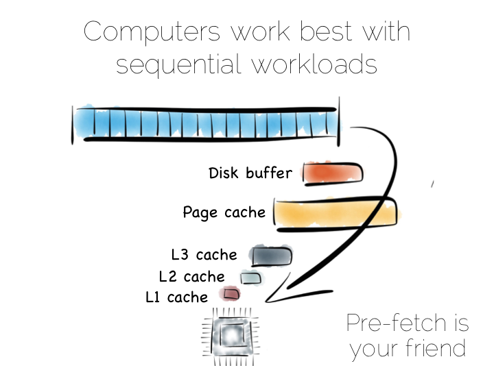
In a somewhat abstract sense, when we’re dealing with data, we’re really just arranging locality. Locality to the CPU. Locality to the other data we need. Accessing data sequentially is an important component of this. Computers are just good at sequential operations. Sequential operations can be predicted.
If you’re taking data from disk sequentially it’ll be pre-fetched into the disk buffer, the page cache and the different levels of CPU caching. This has a significant effect on performance. But it does little to help the addressing of data at random, be it in main memory, on disk or over the network. In fact pre-fetching actually hinders random workloads as the various caches and frontside bus fill with data which is unlikely to be used.
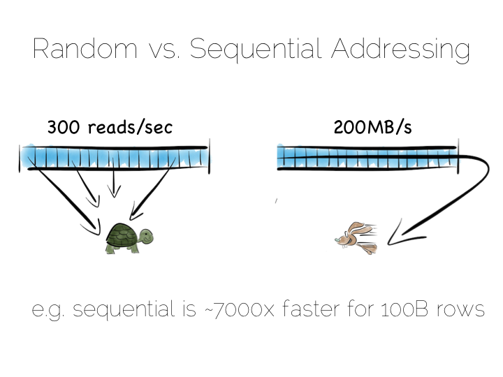
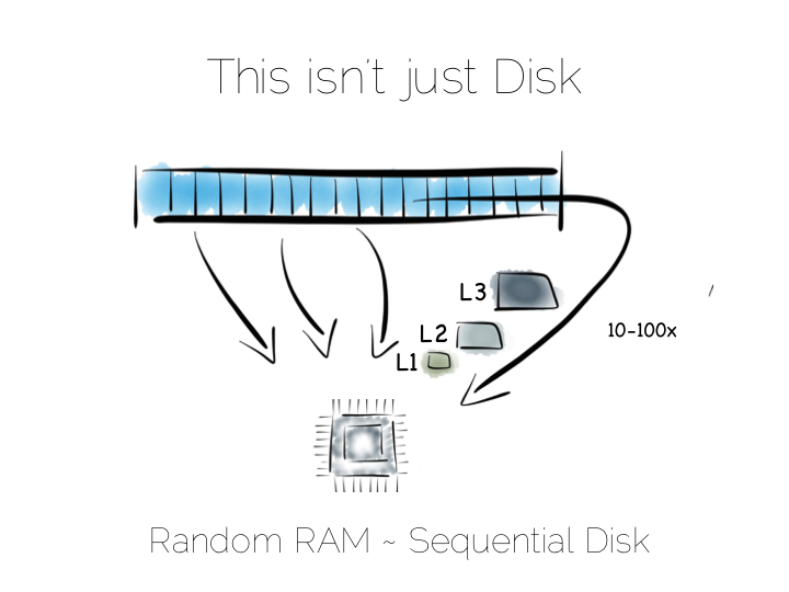
So whilst disk is somewhat renowned for its slow performance, main memory is often assumed to simply be fast. This is not as ubiquitously true as people often think. There are one to two orders of magnitude between random and sequential main memory workloads. Use a language that manages memory for you and things generally get a whole lot worse.
Streaming data sequentially from disk can actually outperform randomly addressed main memory. So disk may not always be quite the tortoise we think it is, at least not if we can arrange sequential access. SSD’s, particularly those that utilise PCIe, further complicate the picture as they demonstrate different tradeoffs, but the caching benefits of the two access patterns remain, regardless.
So lets imagine, as a simple thought experiment, that we want to create a very simple database. We’ll start with the basics: a file.
We want to keep writes and reads sequential, as it works well with the hardware. We can append writes to the end of the file efficiently. We can read by scanning the the file in its entirety. Any processing we wish to do can happen as the data streams through the CPU. We might filter, aggregate or even do something more complex. The world is our oyster!
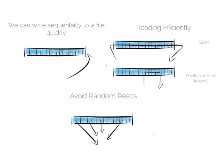
So what about data that changes, updates etc?
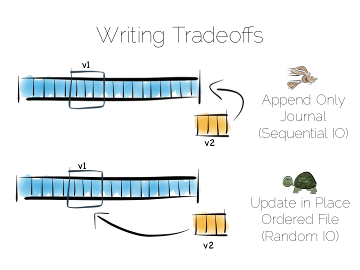
We have a couple of options. We could update the value in place. We’d need to use fixed width fields for this, but that’s ok for our little thought experiment. But update in place would mean random IO. We know that’s not good for performance.
Alternatively we could just append updates to the end of the file and deal with the superseded values when we read it back.
So we have our first tradeoff. Append to a ‘journal’ or ‘log’, and reap the benefits of sequential access. Alternatively if we use update in place we’ll be back to 300 or so writes per second, assuming we actually flush through to the underlying media.
Now in practice of course reading the file, in its entirety, can be pretty slow. We’ll only need to get into GB’s of data and the fastest disks will take seconds. This is what a database does when it ends up table scanning.
Also we often want something more specific, say customers named “bob”, so scanning the whole file would be overkill. We need an index.
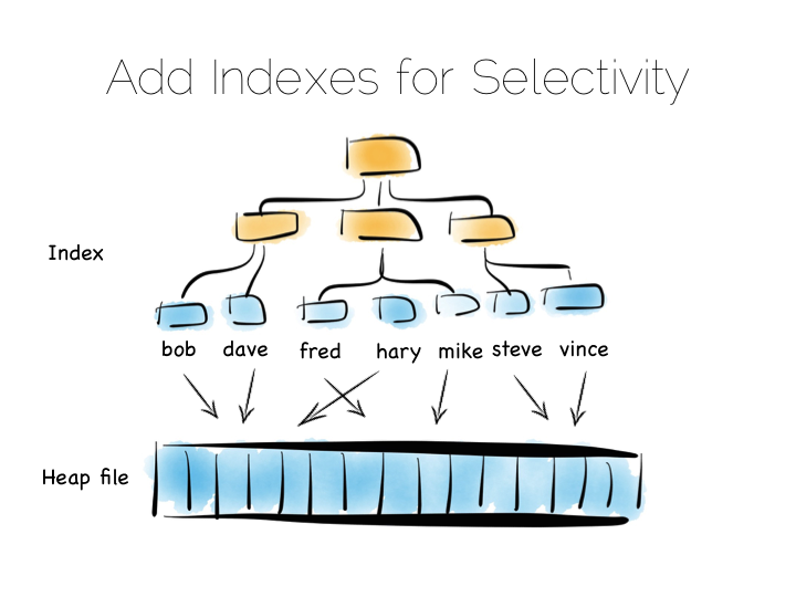
Now there are lots of different types of indexes we could use. The simplest would be an ordered array of fixed-width values, in this case customer names, held with the corresponding offsets in the heap file. The ordered array could be searched with binary search. We could also of course use some form of tree, bitmap index, hash index, term index etc. Here we’re picturing a tree.
The thing with indexes like this is that they impose an overarching structure. The values are deliberately ordered so we can access them quickly when we want to do a read. The problem with the overarching structure is that it necessitates random writes as data flows in. So our wonderful, write optimised, append only file must be augmented by writes that scatter-gun the filesystem. This is going to slow us down.
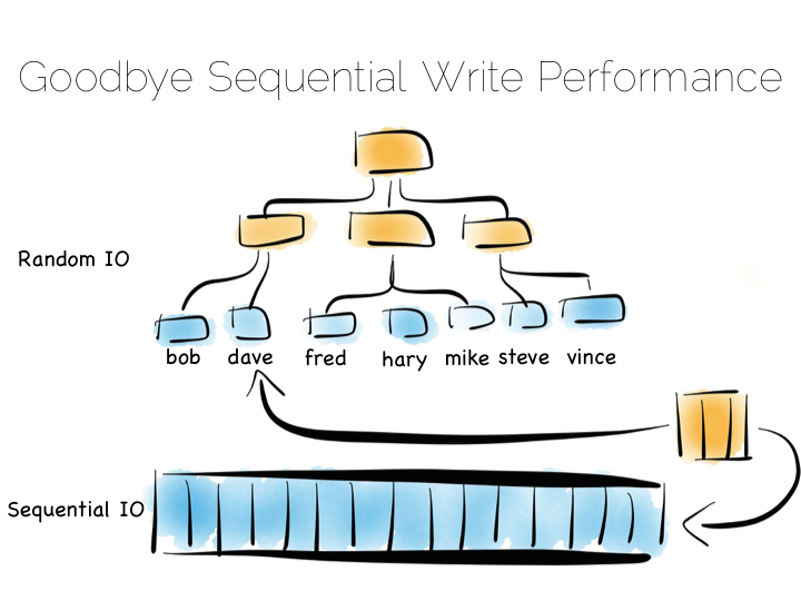
Anyone who has put lots of indexes on a database table will be familiar with this problem. If we are using a regular rotating hard drive, we might run 1,000s of times slower if we maintain disk integrity of an index in this way.
Luckily there are a few ways around this problem. Here we are going to discuss three. These represent three extremes, and they are in truth simplifications of the real world, but the concepts are useful when we consider larger compositions.
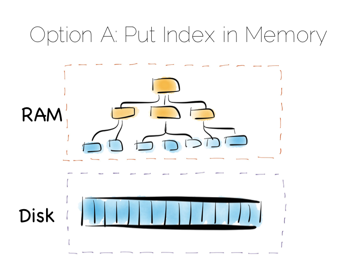
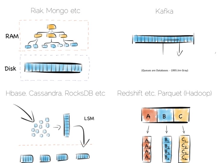
Our first option is simply to place the index in main memory. This will compartmentalise the problem of random writes to RAM. The heap file stays on disk.
This is a simple and effective solution to our random writes problem. It is also one used by many real databases. MongoDB, Cassandra, Riak and many others use this type of optimisation. Often memory mapped files are used.
However, this strategy breaks down if we have far more data than we have main memory. This is particularly noticeable where there are lots of small objects. Our index would get very large. Thus our storage becomes bounded by the amount of main memory we have available. For many tasks this is fine, but if we have very large quantities of data this can be a burden.
A popular solution is to move away from having a single ‘overarching’ index. Instead we use a collection of smaller ones.
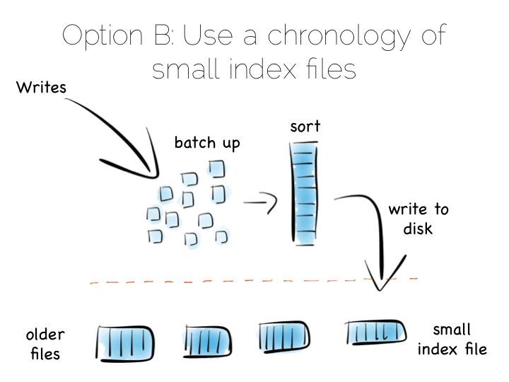
This is a simple idea. We batch up writes in main memory, as they come in. Once we have sufficient – say a few MB’s – we sort them and write them to disk as an individual mini-index. What we end up with is a chronology of small, immutable index files.
So what was the point of doing that? Our set of immutable files can be streamed sequentially. This brings us back to a world of fast writes, without us needing to keep the whole index in memory. Nice!
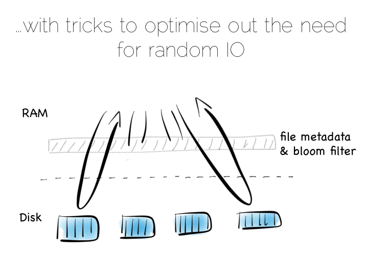
Of course there is a downside to this approach too. When we read, we have to consult the many small indexes individually. So all we have really done is shift the problem of RandomIO from writes onto reads. However this turns out to be a pretty good tradeoff in many cases. It’s easier to optimise random reads than it is to optimise random writes.
Keeping a small meta-index in memory or using a Bloom Filter provides a low-memory way of evaluating whether individual index files need to be consulted during a read operation. This gives us almost the same read performance as we’d get with a single overarching index whilst retaining fast, sequential writes.
In reality we will need to purge orphaned updates occasionally too, but that can be done with nice sequential reads and writes.
What we have created is termed a Log Structured Merge Tree. A storage approach used in a lot of big data tools such as HBase, Cassandra, Google’s BigTable and many others. It balances write and read performance with comparatively small memory overhead.
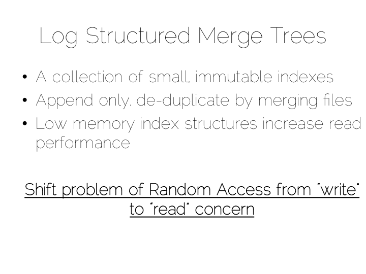
So we can get around the ‘random-write penalty’ by storing our indexes in memory or, alternatively, using a write-optimised index structure like LSM. There is a third approach though. Pure brute force.
Think back to our original example of the file. We could read it in its entirety. This gave us many options in terms of how we go about processing the data within it. The brute force approach is simply to hold data by column rather than by row. This approach is termed Columnar or Column Oriented.
(It should be noted that there is an unfortunate nomenclature clash between true column stores and those that follow the Big Table pattern. Whilst they share some similarities, in practice they are quite different. It is wise to consider them as different things.)
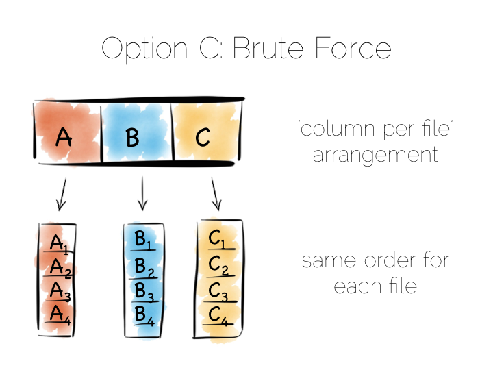
Column Orientation is another simple idea. Instead of storing data as a set of rows, appended to a single file, we split each row by column. We then store each column in a separate file. When we read we only read the columns we need.
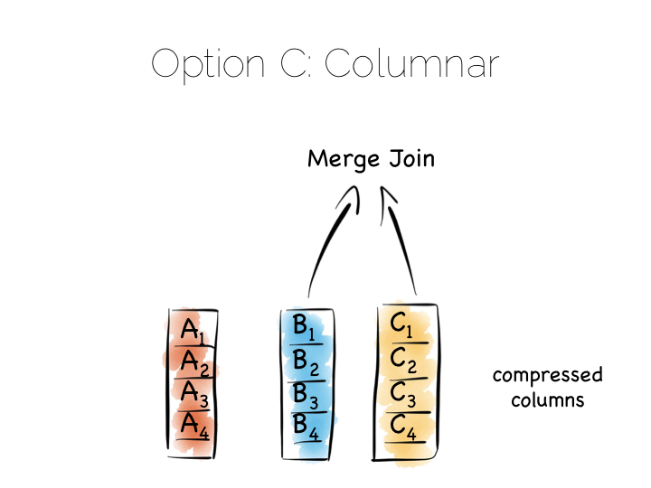
We keep the order of the files the same, so row N has the same position (offset) in each column file. This is important because we will need to read multiple columns to service a single query, all at the same time. This means ‘joining’ columns on the fly. If the columns are in the same order we can do this in a tight loop which is very cache- and cpu-efficient. Many implementations make heavy use of vectorisation to further optimise throughput for simple join and filter operations.
Writes can leverage the benefits of being append-only. The downside is that we now have many files to update, one for every column in every individual write to the database. The most common solution to this is to batch writes in a similar way to the one used in the LSM approach above. Many columnar databases also impose an overall order to the table as a whole to increase their read performance for one chosen key.
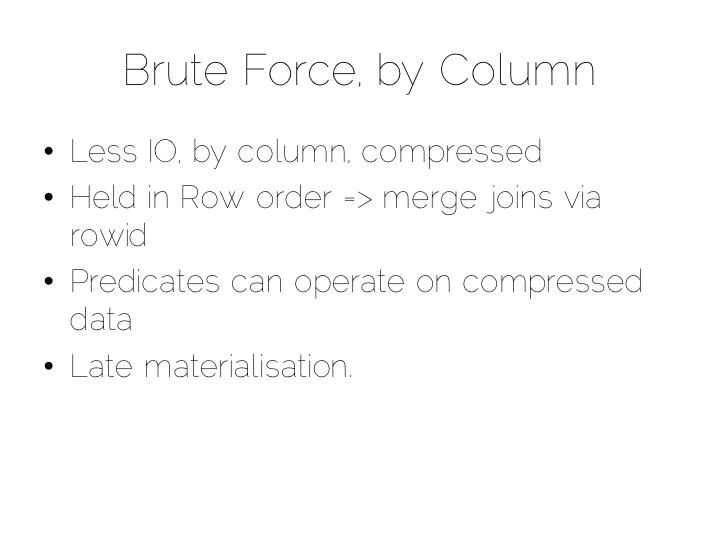
By splitting data by column we significantly reduce the amount of data that needs to be brought from disk, so long as our query operates on a subset of all columns.
In addition to this, data in a single column generally compresses well. We can take advantage of the data type of the column to do this, if we have knowledge of it. This means we can often use efficient, low cost encodings such as run-length, delta, bit-packed etc. For some encodings predicates can be used directly on the compressed stream too.
The result is a brute force approach that will work particularly well for operations that require large scans. Aggregate functions like average, max, min, group by etc are typical of this.
This is very different to using the ‘heap file & index’ approach we covered earlier. A good way to understand this is to ask yourself: what is the difference between a columnar approach like this vs a ‘heap & index’ where indexes are added to every field?
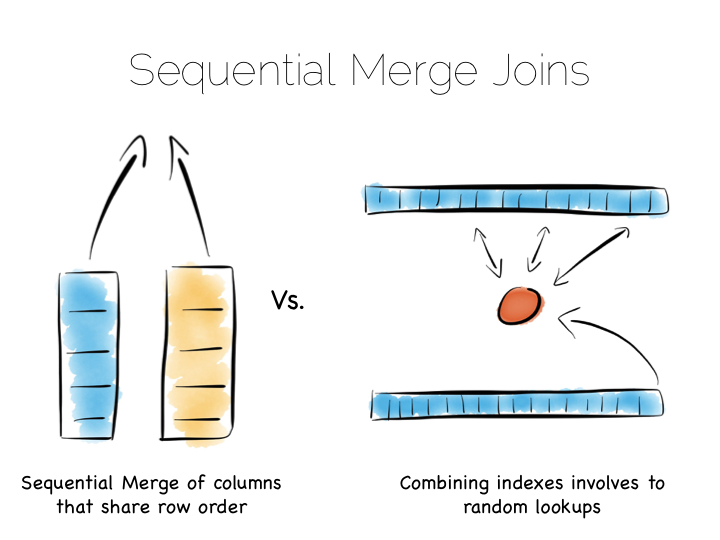
The answer to this lies in the ordering of the index files. BTrees etc will be ordered by the fields they index. Joining the data in two indexes involves a streaming operation on one side, but on the other side the index lookups have to read random positions in the second index. This is generally less efficient than joining two indexes (columns) that retain the same ordering. Again we’re leveraging sequential access.
So many of the best technologies which we may want to use as components in a data platform will leverage one of these core efficiencies to excel for a certain set of workloads.
Storing indexes in memory, over a heap file, is favoured by many NoSQL stores such as Riak, Couchbase or MongoDB as well as some relational databases. It’s a simple model that works well.
Tools designed to work with larger data sets tend to take the LSM approach. This gives them fast ingestion as well as good read performance using disk based structures. HBase, Cassandra, RocksDB, LevelDB and even Mongo now support this approach.
Column-per-file engines are used heavily in MPP databases like Redshift or Vertica as well as in the Hadoop stack using Parquet. These are engines for data crunching problems that require large traversals. Aggregation is the home ground for these tools.
Other products like Kafka apply the use of a simple, hardware efficient contract to messaging. Messaging, at its simplest, is just appending to a file, or reading from a predefined offset. You read messages from an offset. You go away. You come back. You read from the offset you previously finished at. All nice sequential IO.
This is different to most message oriented middleware. Specifications like JMS and AMQP require the addition of indexes like the ones discussed above, to manage selectors and session information. This means they often end up performing more like a database than a file. Jim Gray made this point famously back in his 1995 publication Queue’s are Databases.
So all these approaches favour one tradeoff or other, often keeping things simple, and hardware sympathetic, as a means of scaling.
So we’ve covered some of the core approaches to storage engines. In truth we made some simplifications. The real world is a little more complex. But the concepts are useful nonetheless.
Scaling a data platform is more than just storage engines though. We need to consider parallelism.

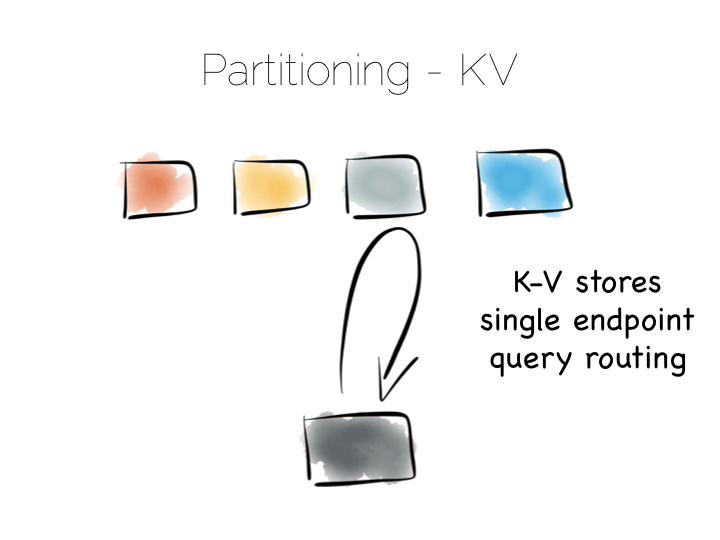
When distributing data over many machines we have two core primitives to play with: partitioning and replication. Partitioning, sometimes called sharding, works well both for random access and brute force workloads.
If a hash-based partitioning model is used the data will be spread across a number of machines using a well-known hash function. This is similar to the way a hash table works, with each bucket being held on a different machine.
The result is that any value can be read by going directly to the machine that contains the data, via the hash function. This pattern is wonderfully scalable and is the only pattern that shows linear scalability as the number of client requests increases. Requests are isolated to a single machine. Each one will be served by just a single machine in the cluster.
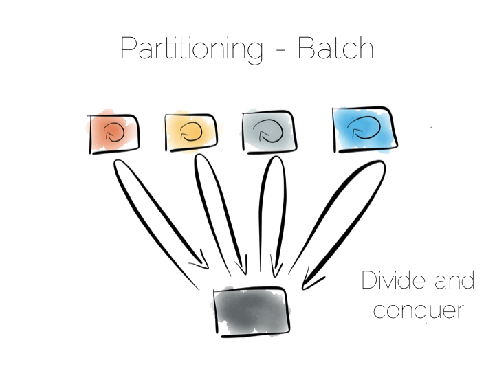
We can also use partitioning to provide parallelism over batch computations, for example aggregate functions or more complex algorithms such as those we might use for clustering or machine learning. The key difference is that we exercise all machines at the same time, in a broadcast manner. This allows us to solve a large computational problem in a much shorter time, using a divide and conquer approach.
Batch systems work well for large problems, but provide little concurrency as they tend to exhaust the resources on the cluster when they execute.
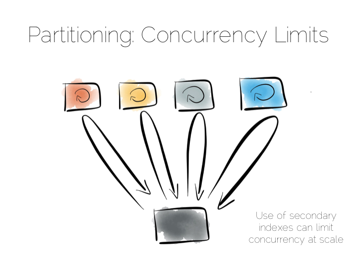
So the two extremes are pretty simple: Directed access at one end. Broadcast, divide and conquer at the other. Where we need to be careful is in the middle ground that lies between the two. A good example of this is the use of secondary indexes in NoSQL stores that span many machines.
A secondary index is an index that isn’t on the primary key. This means the data will not be partitioned by the values in the index. Directed routing via a hash function is no longer an option. We have to broadcast requests to all machines. This limits concurrency. Every node must be involved in every query.
For this reason many key value stores have resisted the temptation to add secondary indexes, despite their obvious use. HBase and Voldemort are examples of this. But many others do expose them, MongoDB, Cassandra, Riak etc. This is good as secondary indexes are useful. But it’s important to understand the effect they will have on the overall concurrency of the system.
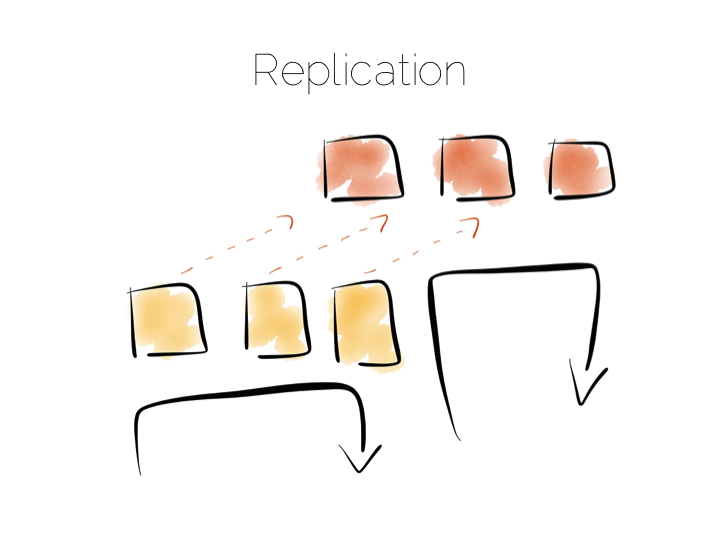
The route out of this concurrency bottleneck is replication. You’ll probably be familiar with replication either from using async slave databases or from replicated NoSQL stores like Mongo or Cassandra.
In practice replicas can be invisible (used only for recovery), read only (adding concurrency) or read-write (adding availability under network partitions). Which of these you choose will trade off against the consistency of the system. This is simply the application of CAP theorem (although cap theorem also may not be as simple as you think).
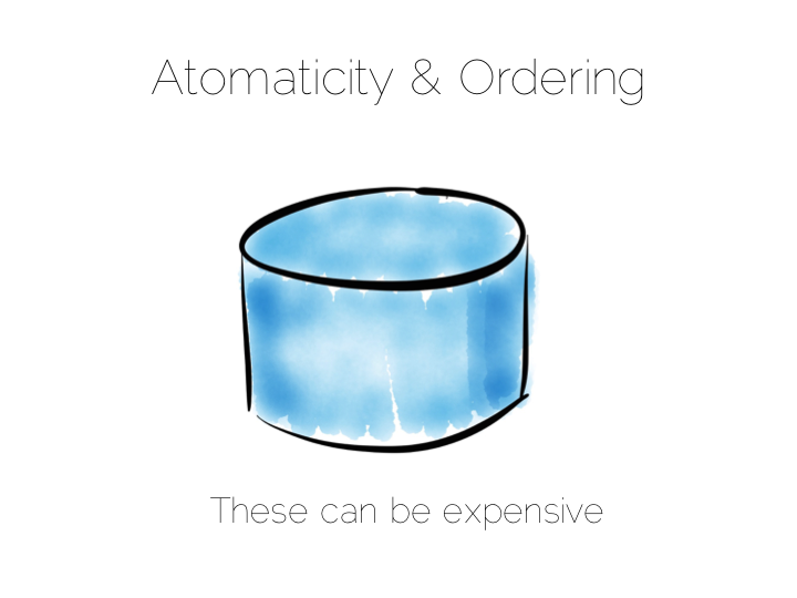
This tradeoff with consistency* brings us to an important question. When does consistency matter?
Consistency is expensive. In the database world ACID is guaranteed by linearisabilty. This is essentially ensuring that all operations appear to occur in sequential order. It turns out to be a pretty expensive thing. In fact it’s prohibitive enough that many databases don’t offer it as an isolation level at all. Those that do, rarely set it as the default.
Suffice to say that if you apply strong consistency to a system that does distributed writes you’ll likely end up in tortoise territory.
(* note the term consistency has two common usages. The C in ACID and the C in CAP. They are unfortunately not the same. I’m using the CAP definition: all nodes see the same data at the same time)
The solution to this consistency problem is simple. Avoid it. If you can’t avoid it isolate it to as few writers and as few machines as possible.
Avoiding consistency issues is often quite easy, particularly if your data is an immutable stream of facts. A set of web logs is a good example. They have no consistency concerns as they are just facts that never change.
There are other use cases which do necessitate consistency though. Transferring money between accounts is an oft used example. Non-commutative actions such as applying discount codes is another.
But often things that appear to need consistency, in a traditional sense, may not. For example if an action can be changed from a mutation to a new set of associated facts we can avoid mutable state. Consider marking a transaction as being potentially fraudulent. We could update it directly with the new field. Alternatively we could simply use a separate stream of facts that links back to the original transaction.
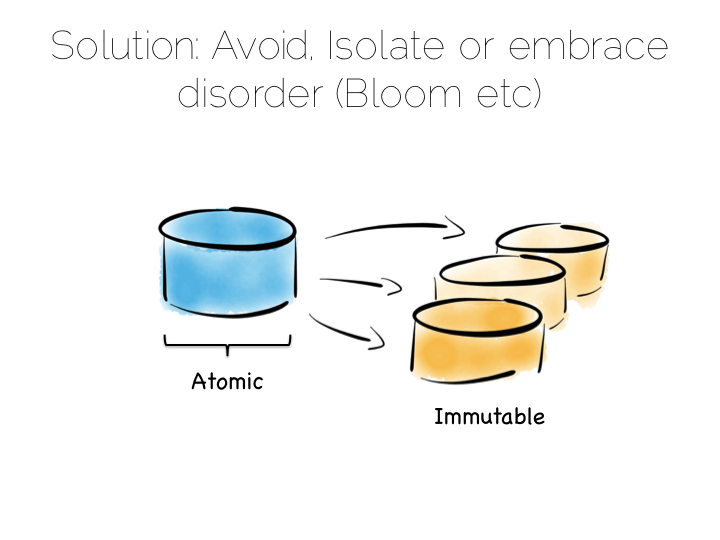
So in a data platform it’s useful to either remove the consistency requirement altogether, or at least isolate it. One way to isolate is to use the single writer principal, this gets you some of the way. Datomic is a good example of this. Another is to physically isolate the consistency requirement by splitting mutable and immutable worlds.
Approaches like Bloom/CALM extend this idea further by embracing the concept of disorder by default, imposing order only when necessary.
So those were some of the fundamental tradeoffs we need to consider. Now how to we pull these things together to build a data platform?

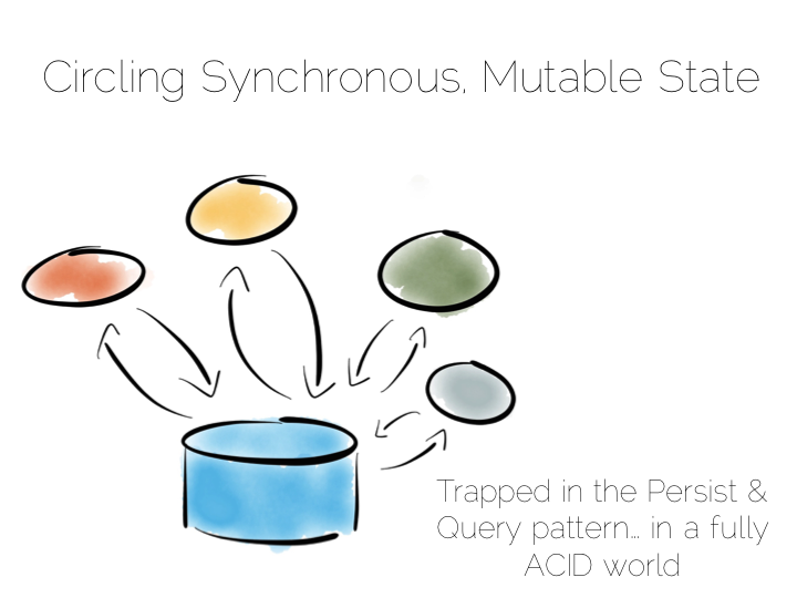
A typical application architecture might look something like the below. We have a set of processes which write data to a database and read it back again. This is fine for many simple workloads. Many successful applications have been built with this pattern. But we know it works less well as throughput grows. In the application space this is a problem we might tackle with message-passing, actors, load balancing etc.
The other problem is this approach treats the database as a black box. Databases are clever software. They provide a huge wealth of features. But they provide few mechanisms for scaling out of an ACID world. This is a good thing in many ways. We default to safety. But it can become an annoyance when scaling is inhibited by general guarantees which may be overkill for the requirements we have.
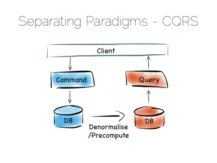
The simplest route out of this is CQRS (Command Query Responsibility Segregation).
Another very simple idea. We separate read and write workloads. Writes go into something write-optimised. Something closer to a simple journal file. Reads come from something read-optimised. There are many ways to do this, be it tools like Goldengate for relational technologies or products that integrate replication internally such as Replica Sets in MongoDB.
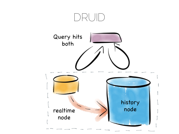
Many databases do something like this under the hood. Druid is a nice example. Druid is an open source, distributed, time-series, columnar analytics engine. Columnar storage works best if we input data in large blocks, as the data must be spread across many files. To get good write performance Druid stores recent data in a write optimised store. This is gradually ported over to the read optimised store over time.
When Druid is queried the query routes to both the write optimised and read optimised components. The results are combined (‘reduced’) and returned to the user. Druid uses time, marked on each record, to determine ordering.
Composite approaches like this provide the benefits of CQRS behind a single abstraction.
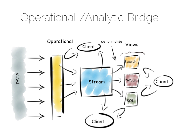
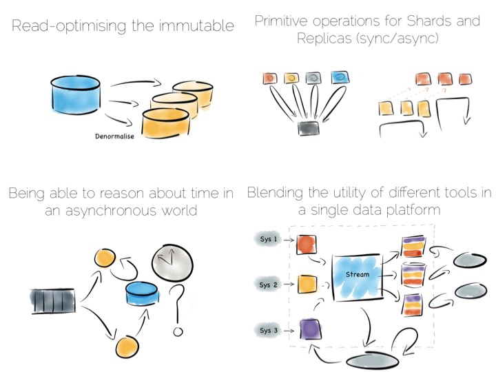
Another similar approach is to use an Operational/Analytic Bridge. Read- and write-optimised views are separated using an event stream. The stream of state is retained indefinitely, so that the async views can be recomposed and augmented at a later date by replaying.
So the front section provides for synchronous reads and writes. This can be as simple as immediately reading data that was written or as complex as supporting ACID transactions.
The back end leverages asynchronicity, and the advantages of immutable state, to scale offline processing through replication, denormalisation or even completely different storage engines. The messaging-bridge, along with joining the two, allows applications to listen to the data flowing through the platform.
As a pattern this is well suited to mid-sized deployments where there is at least a partial, unavoidable requirement for a mutable view.
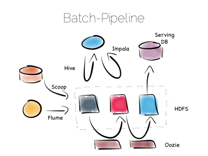
If we are designing for an immutable world, it’s easier to embrace larger data sets and more complex analytics. The batch pipeline, one almost ubiquitously implemented with the Hadoop stack, is typical of this.
The beauty of the Hadoop stack comes from it’s plethora of tools. Whether you want fast read-write access, cheap storage, batch processing, high throughput messaging or tools for extracting, processing and analysing data, the Hadoop ecosystem has it all.
The batch pipeline architecture pulls data from pretty much any source, push or pull. Ingests it into HDFS then processes it to provide increasingly optimised versions of the original data. Data might be enriched, cleansed, denormalised, aggregated, moved to a read optimised format such as Parquet or loaded into a serving layer or data mart. Data can be queried and processed throughout this process.
This architecture works well for immutable data, ingested and processed in large volume. Think 100’s of TBs (although size alone isn’t a great metric). The evolution of this architecture will be slow though. Straight-through timings are often measured in hours.
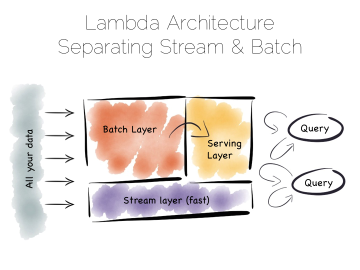
The problem with the Batch Pipeline is that we often don’t want to wait hours to get a result. A common solution is to add a streaming layer aside it. This is sometimes referred to as the Lambda Architecture.
The Lambda Architecture retains a batch pipeline, like the one above, but it circumvents it with a fast streaming layer. It’s a bit like building a bypass around a busy town. The streaming layer typically uses a streaming processing tool such as Storm or Samza.
The key insight of the Lambda Architecture is that we’re often happy to have an approximate answer quickly, but we would like an accurate answer in the end.
So the streaming layer bypasses the batch layer providing the best answers it can within a streaming window. These are written to a serving layer. Later the batch pipeline computes an accurate data and overwrites the approximation.
This is a clever way to balance accuracy with responsiveness. Some implementations of this pattern suffer if the two branches end up being dual coded in stream and batch layers. But it is often possible to simply abstract this logic into common libraries that can be reused, particularly as much of this processing is often written in external libraries such as Python or R anyway. Alternatively systems like Spark provide both stream and batch functionality in one system (although the streams in Spark are really micro-batches).
So this pattern again suits high volume data platforms, say in the 100TB range, that want to combine streams with existing, rich, batch based analytic function.
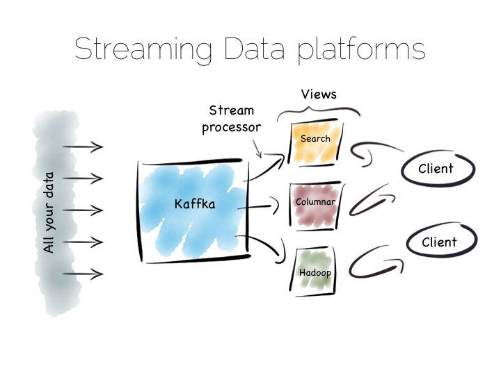
There is another approach to this problem of slow data pipelines. It’s sometimes termed the Kappa architecture. I actually thought this name was ‘tongue in cheek’ but I’m now not so sure. Whichever it is, I’m going to use the term Stream Data Platform, which is a term in use also.
Stream Data Platform’s flip the batch pattern on its head. Rather than storing data in HDFS, and refining it with incremental batch jobs, the data is stored in a scale out messaging system, or log, such as Kafka. This becomes the system of record and the stream of data is processed in real time to create a set of tertiary views, indexes, serving layers or data marts.
This is broadly similar to the streaming layer of the Lambda architecture but with the batch layer removed. Obviously the requirement for this is that the messaging layer can store and vend very large volumes of data and there is a sufficiently powerful stream processor to handle the processing.
There is no free lunch so, for hard problems, Stream Data Platform’s will likely run no faster than an equivalent batch system, but switching the default approach from ‘store and process’ to ‘stream and process’ can provide greater opportunity for faster results.
Finally, the Stream Data Platform approach can be applied to the problem of ‘application integration’. This is a thorny and difficult problem that has seen focus from big vendors such as Informatica, Tibco and Oracle for many years. For the most part results have been beneficial, but not transformative. Application integration remains a topic looking for a real workable solution.
Stream Data Platform’s provide an interesting potential solution to this problem. They take many of the benefits of an O/A bridge – the variety of asynchronous storage formats and ability to recreate views – but leave the consistency requirement isolated in, often existing sources:
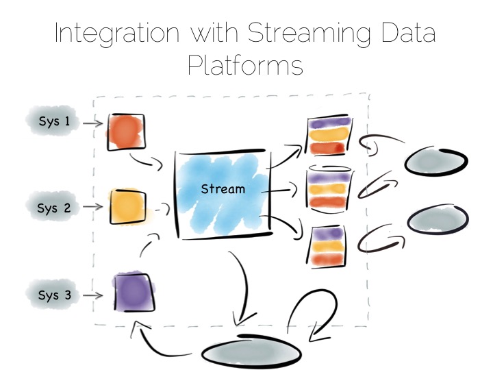
With the system of record being a log it’s easy to enforce immutability. Products like Kafka can retain enough volume and throughput, internally, to be used as a historic record. This means recovery can be a process of replaying and regenerating state, rather than constantly checkpointing.
Similarly styled approaches have been taken before in a number of large institutions with tools such as Goldengate, porting data to enterprise data warehouses or more recently data lakes. They were often thwarted by a lack of throughput in the replication layer and the complexity of managing changing schemas. It seems unlikely the first problem will continue. As for the later problem though, the jury is still out.
~
So we started with locality. With sequential addressing for both reads and writes. This dominates the tradeoffs inside the components we use. We looked at scaling these components out, leveraging primitives for both sharding and replication. Finally we rebranded consistency as a problem we should isolate in the platforms we build.
But data platforms themselves are really about balancing the sweet-spots of these individual components within a single, holistic form. Incrementally restructuring. Migrating the write-optimised to the read-optimised. Moving from the constraints of consistency to the open plains of streamed, asynchronous, immutable state.
This must be done with a few things in mind. Schemas are one. Time, the peril of the distributed, asynchronous world, is another. But these problems are manageable if carefully addressed. Certainly the future is likely to include more of these things, particularly as tooling, innovated in the big data space, percolates into platforms that address broader problems, both old and new.
~
THINGS WE LIKE
Upside Down Databases: Bridging the Operational and Analytic Worlds with Streams
Tuesday, April 7th, 2015
Remember the days when people would write entire applications, embedded inside a database? It seems a bit crazy now when you think about it. Imagine writing an entire application in SQL. I worked on a beast like that, very briefly, in the late 1990s. It had a few shell scripts but everything else was SQL. Everything. Suffice to say it wasn’t much fun – you can probably imagine – but there was a slightly perverse simplicity to the whole thing.
So Martin Kleppmann did a talk recently around the idea of turning databases inside out. I like this idea. It’s a nice way to frame a problem that has lurked unresolved for years. To paraphrase somewhat… databases do very cool stuff: caching, indexes, replication, materialised views. These are very cool things. They do them well too. It’s a shame that they’re locked in a world dislocated from general consumer programs.
There are also a few things missing, like databases don’t really do events, streams, messaging, whatever you want to call it. Some newer ones do, but none cover what you might call ‘general purpose’ streams. This means the query-driven paradigm often leaks into the application space. Applications end up circling around centralised mutable state. Whilst there are valid use cases for this, the rigid and synchronous world produced can be counterproductive for many types of programs.
So it’s interesting to look at the pros and cons of externalising caches, indexes, materialised views and asynchronous streams of state. I got to see some of these ideas play out in a data platform built for a large financial institution. It used messaging as the system of record. It also employed synchronous and asynchronous views. These could be generated, and regenerated, from this event stream.
The approach had some nice side effects which we didn’t originally anticipate. Making the system of record an event stream was actually born somewhat from necessity. The front of the system used a data grid as a consolidation point. Data grids need external persistence. We wanted the back end to support analytics. Analytic systems work best when writes are batched, so we needed something to buffer the two. Something that would scale out disk writes linearly with the sharded data grid. Topic based messaging seemed like a good fit. Clients needed notifications anyway.
This led to some interesting properties. The front end provided a near term, consistent view. Clients could collaborate around it. It could be scaled out horizontally by adding shards. At the back, everything was asynchronous and immutable. This meant it was easy to scale with replicas. Creating another replica is relatively simple when your system of record is an event stream.
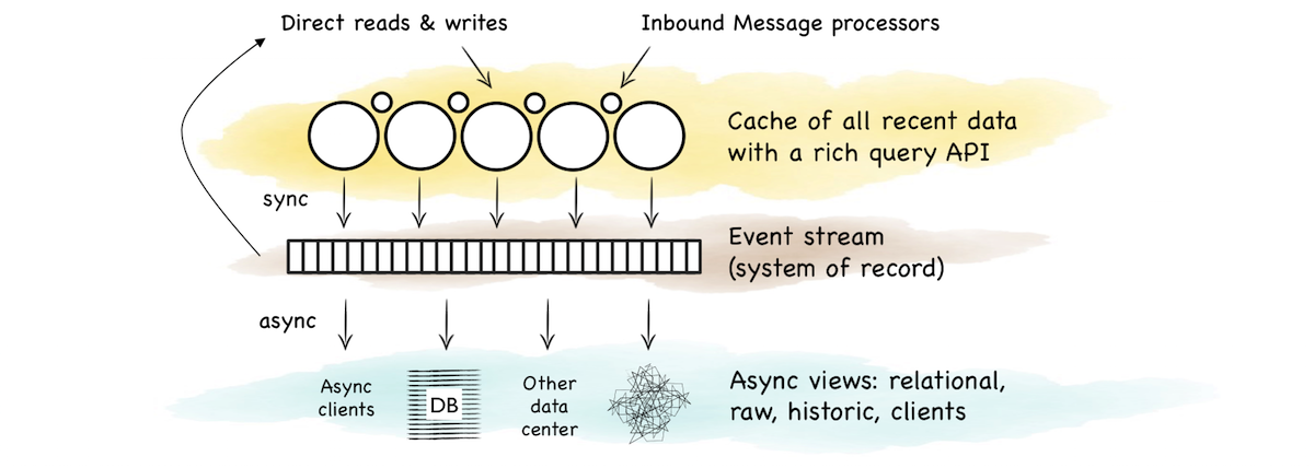
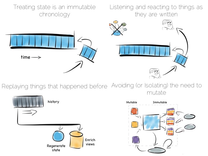
The event stream tied the two together. It was the bridge between the operational and analytic sections. A stream for clients to fork directly or as a firehose to create another view.
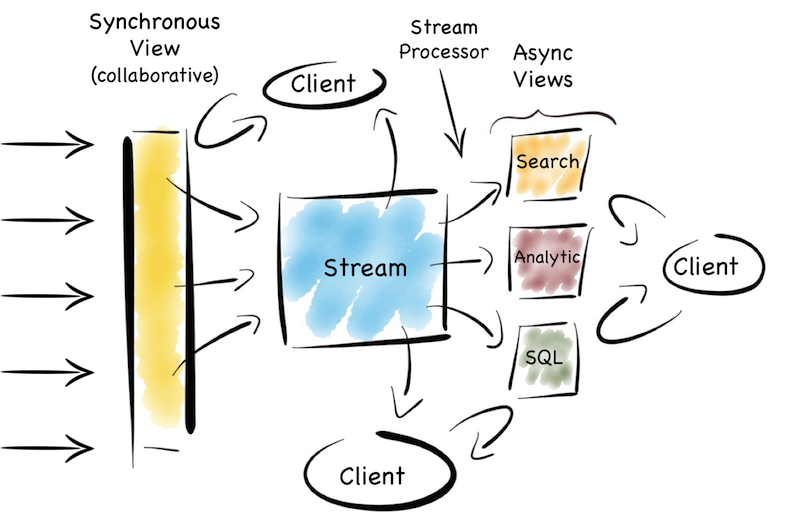
So this is a pattern that bridges operational and analytic worlds. The operational layer provides state management for recent data. The stream buffers these changes as a log. The log forms a replayable, immutable, chronology. Views are created via functions that operate on the stream. The flow of versions is ubiquitous and unidirectional. This creates a nice synergy between stream and query. Data in motion and data at rest just become different points of reference.
After a couple of years a few things became apparent. The first was that scaling the consistent layer at the front was harder than replicating at the back. The problem was that most users ran fairly complex queries, rather than doing key-based access. General queries & processing doesn’t scale out linearly in a shared nothing model, particularly when you get to hundreds of nodes. Only key based access has that grace. You can scale out, but you get diminishing returns as you grow.
The views at the back were, by contrast, easier to scale, at least for simple analytics, ad hoc queries and report-style stuff which big organisations have lots of. This was quite nice.
At it’s essence this is just CQRS. But it’s partial CQRS. Writes at the front are separated from reads at the back. But if a writer needs to read the current state, say to support conditional changes or non-commutative actions, then a mutable view is available*. Conversely the back end leverages the benefits of an immutable, append only world.
So this offloads reads from the contended front section. But it also means the back section can ‘specialise’. This is what you might refer to as a set of materialised views or indexes. Different data arrangements, with different populations, in different places, using different indexing strategies or even different technologies altogether.
Now there are other good ways to achieve this. Simple database replication (relationally or nosql) is a good route. Relational folk would do this with the data mart pattern. Some newer products, particularly nosql ones (Mongo etc), provide both replication and sharding as first class citizens, meaning a single technology can provide a good proportion of this function out of the box. But it’s harder to get truly broad utility from a single product. These days we often want to combine a range of search, analytic, relational and routable (selector based) messaging technologies to leverage their respective sweet spots.
So integrating a set of technologies into a single data platform helps play to such functional sweet spots whilst making the problems of polyglotic persistence more manageable.
An important element of this is the ability to generate, regenerate and widen views, on demand, from the original stream. This is analogous to the way a database creates materialised views, changing them as you alter the view definition. Hadoop pipelines often do this too, in one form or another. But if you don’t address this holistically problems will likely ensue. You’ll end up altering views independently, in an ad hoc manner, rather than appending to, and replaying, the stream. This leads down a path of divergence. Pain will follow.
So the trick, at least for me, is how this is all tied together. A synchronous writeable view at the front. A range of different read-only views at the back, running asynchronous to one another. An event stream tying it all together with a single journal of state. Side effect free functions that (re)generate different views from the stream. A spout for programs to listen and interact. All wrapped up in a single data platform. A single joined up unit.
Martin suggests, in his original talk, using the Samza stack to manage views like these with Kafka providing the log. This seems a good place to start today. Kafka’s bare-boned approach certainly removes many of the scalability barriers seen in JMS/AMQP implementations, albeit at the cost of some utility.
There are, of course, a plethora of little devils lurking in the detail. There are also a number of points that I skimmed over here. I’m not sure that I’d use a data grid again. In fact I’d argue that the single collaboration point isn’t always necessary*. Time synchronisation across asynchronous views can cause problems. Replaying functions on a historical stream of state is also pretty tricky, particularly as time passes and inbound data formats change. This deserves a post of its own. Finally scaling traditional messaging systems, even using topics, becomes painful, particularly when message selectors are used.
So a solution of this type needs a fairly beefy use case to warrant the effort needed to sew it all together. You wouldn’t use it for a small web app, but it would work well for a large team, division or small company. Ours was a fairly hefty central data programme. But it’s easier today than it was five years ago, and it’ll get easier still. Of that I’m sure.
So it seems unlikely we’ll go back to writing entire applications inside a ‘database’. The world doesn’t really work so well that way. Thankfully, it seems even less likely we’ll go back to writing applications in SQL. But having infrastructure that leverages the separation of mutable and immutable state, synchronicity and asynchronicity. That synergises stream and query. That is a good thing. That gets us to a better place. That, I think, is a pretty nice place to be.
—/—
* Whether you need a fast or consistent, collaborative view, to manage stateful changes, is something worth carefully considering. Many use cases simply collect, process and produce a result. That’s to say they avoid updates, and can live, instead, in a world of immutable values. This means they can neglect the consistent, temporal context needed to update data. This is a fairly deep topic so all I’ll say here is, if you can make do with an append only, immutable data, avoid having a synchronous, consistent view.
Log Structured Merge Trees
Saturday, February 14th, 2015
It’s nearly a decade since Google released its ‘Big Table’ paper. One of the many cool aspects of that paper was the file organisation it uses. The approach is more generally known as the Log Structured Merge Tree, after this 1996 paper, although the algorithm described there differs quite significantly from most real-world implementations.
LSM is now used in a number of products as the main file organisation strategy. HBase, Cassandra, LevelDB, SQLite, even MongoDB 3.0 comes with an optional LSM engine, after it’s acquisition of Wired Tiger.
What makes LSM trees interesting is their departure from binary tree style file organisations that have dominated the space for decades. LSM seems almost counter intuitive when you first look at it, only making sense when you closely consider how files work in modern, memory heavy systems.
Some Background
In a nutshell LSM trees are designed to provide better write throughput than traditional B+ tree or ISAM approaches. They do this by removing the need to perform dispersed, update-in-place operations.
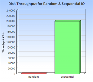 So why is this a good idea? At its core it’s the old problem of disks being slow for random operations, but fast when accessed sequentially. A gulf exists between these two types of access, regardless of whether the disk is magnetic or solid state or even, although to a lesser extent, main memory.
The figures in this ACM report here/here make the point well. They show that, somewhat counter intuitively, sequential disk access is faster than randomly accessing main memory. More relevantly they also show sequential access to disk, be it magnetic or SSD, to be at least three orders of magnitude faster than random IO. This means random operations are to be avoided. Sequential access is well worth designing for.
So with this in mind lets consider a little thought experiment: if we are interested in write throughput, what is the best method to use? A good starting point is to simply append data to a file. This approach, often termed logging, journaling or a heap file, is fully sequential so provides very fast write performance equivalent to theoretical disk speeds (typically 200-300MB/s per drive).
Benefiting from both simplicity and performance log/journal based approaches have rightfully become popular in many big data tools. Yet they have an obvious downside. Reading arbitrary data from a log will be far more time consuming than writing to it, involving a reverse chronological scan, until the required key is found.
This means logs are only really applicable to simple workloads, where data is either accessed in its entirety, as in the write-ahead log of most databases, or by a known offset, as in simple messaging products like Kafka.
So we need more than just a journal to efficiently perform more complex read workloads like key based access or a range search. Broadly speaking there are four approaches that can help us here: binary search, hash, B+ or external.
- Search Sorted File: save data to a file, sorted by key. If data has defined widths use Binary search. If not use a page index + scan.
- Hash: split the data into buckets using a hash function, which can later be used to direct reads.
- B+: use navigable file organisation such as a B+ tree, ISAM etc.
- External file: leave the data as a log/heap and create a separate hash or tree index into it.
All these approaches improve read performance significantly ( n->O(log(n)) in most). Alas these structures add order and that order impedes write performance, so our high speed journal file is lost along the way. You can’t have your cake and eat it I guess.
An insight that is worth making is that all four of the above options impose some form of overarching structure on the data.
Data is deliberately and specifically placed around the file system so the index can quickly find it again later. It’s this structure that makes navigation quick. Alas the structure must of course be honoured as data is written. This is where we start to degrade write performance by adding in random disk access.
There are a couple of specific issues. Two IOs are needed for each write, one to read the page and one to write it back. This wasn’t the case with our log/journal file which could do it in one.
Worse though, we now need to update the structure of the hash or B+ index. This means updating specific parts of the file system. This is known as update-in-place and requires slow, random IO. This point is important: in-place approaches like this scatter-gun the file system performing update-in-place*. This is limiting.
One common solution is to use approach (4) A index into a journal – but keep the index in memory. So, for example, a Hash Table can be used to map keys to the position (offset) of the latest value in a journal file (log). This approach actually works pretty well as it compartmentalises random IO to something relatively small: the key-to-offset mapping, held in memory. Looking up a value is then only a single IO.
On the other hand there are scalability limits, particularly if you have lots of small values. If your values were just say simple numbers then the index would be larger than the data file itself. Despite this the pattern is a sensible compromise which is used in many products from Riak through to Oracle Coherence.
So this brings us on to Log Structured Merge Trees. LSMs take a different approach to the four above. They can be fully disk-centric, requiring little in memory storage for efficiency, but also hang onto much of the write performance we would tie to a simple journal file. The one downside is slightly poorer read performance when compared to say a B+Tree.
In essence they do everything they can to make disk access sequential. No scatter-guns here!
*A number of tree structures exist which do not require update-in-place. Most popular is the append-only Btree, also know as the copy-on-write tree. These work by overwriting the tree structure, sequentially, at the end of the file each time a write occurs. Relevant parts of the old tree structure, including the top level node, are orphaned. Through this method update-in-place is avoided as the tree sequentially redefines itself over time. This method does however come at the cost: rewriting the structure on every write is verbose. It creates a significant amount of write amplification which is a downside unto itself.
The Base LSM Algorithm
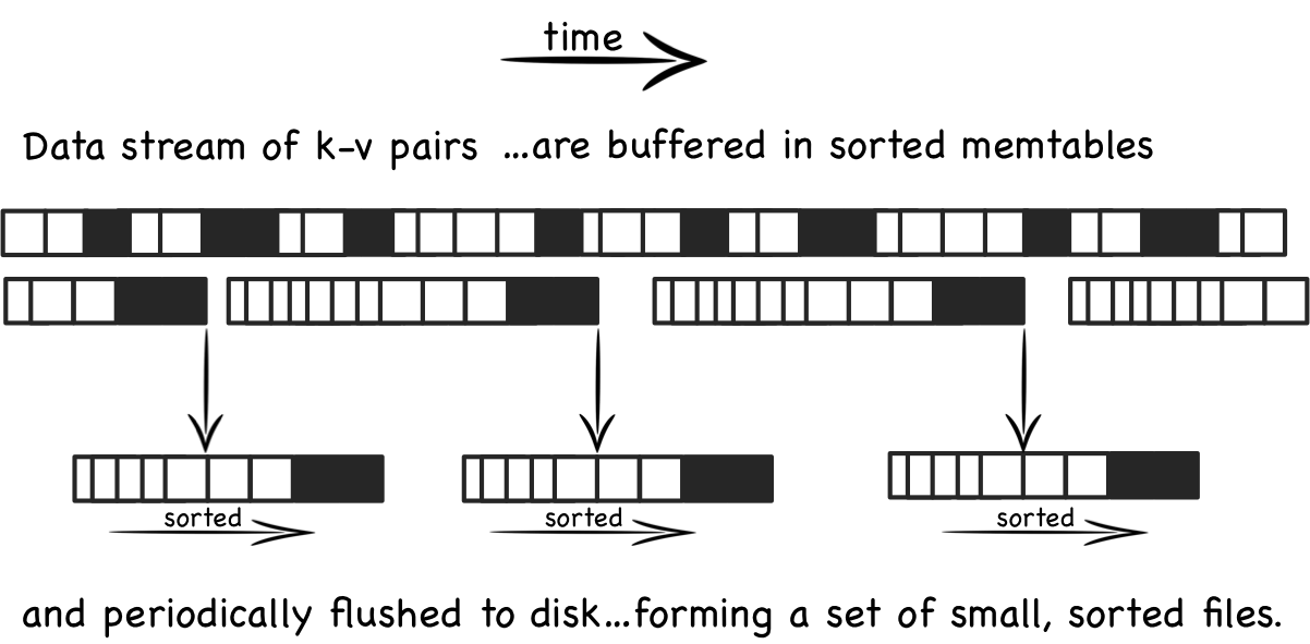
Conceptually the base LSM tree is fairly simple. Instead of having one big index structure (which will either scatter-gun the file system or add significant write amplification) batches of writes are saved, sequentially, to a set of smaller index files. So each file contains a batch of changes covering a short period of time. Each file is sorted before it is written so searching it later will be fast. Files are immutable; they are never updated. New updates go into new files. Reads inspect all files. Periodically files are merged together to keep the number of files down.
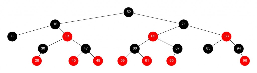
Lets look at this in a little more detail. When updates arrive they are added to an in-memory buffer, which is usually held as a tree (Red-Black etc) to preserve key-ordering. This ‘memtable’ is replicated on disk as a write-ahead-log in most implementations, simply for recovery purposes. When the memtable fills the sorted data is flushed to a new file on disk. This process repeats as more and more writes come in. Importantly the system is only doing sequential IO as files are not edited. New entries or edits simply create successive files (see fig above).
So as more data comes into the system, more and more of these immutable, ordered files are created. Each one representing a small, chronological subset of changes, held sorted.
As old files are not updated duplicate entries are created to supersede previous records (or removal markers). This creates some redundancy initially.
Periodically the system performs a compaction. Compaction selects multiple files and merges them together, removing any duplicated updates or deletions (more on how this works later). This is important both to remove the aforementioned redundancy but, more importantly, to keep a handle on the read performance which degrades as the number of files increases. Thankfully, because the files are sorted, the process of merging the files is quite efficient.
When a read operation is requested the system first checks the in memory buffer (memtable). If the key is not found the various files will be inspected one by one, in reverse chronological order, until the key is found. Each file is held sorted so it is navigable. However reads will become slower and slower as the number of files increases, as each one needs to be inspected. This is a problem.
So reads in LSM trees are slower than their in-place brethren. Fortunately there are a couple of tricks which can make the pattern performant. The most common approach is to hold a page-index in memory. This provides a lookup which gets you ‘close’ to your target key. You scan from there as the data is sorted. LevelDB, RocksDB and BigTable do this with a block-index held at the end of each file. This often works better than straight binary search as it allows the use of variable length fields and is better suited to compressed data.
Even with per-file indexes read operations will still slow as the number of files increases. This is kept in check by periodically merging files together. Such compactions keep the number of files, and hence read performance, within acceptable bounds.
Even with compaction reads will still need to visit many files. Most implementations void this through the use of a Bloom filter. Bloom filters are a memory efficient way of working out whether a file contains a key.
So from a ‘write’ perspective; all writes are batched up and written only in sequential chunks. There is an additional, periodic IO penalty from compaction rounds. Reads however have the potential to touch a large number of files when looking up a single row (i.e. scatter-gun on read). This is simply the way the algorithm works. We’re trading random IO on write for random IO on read. This trade off is sensible if we can use software tricks like bloom filters or hardware tricks like large file caches to optimise read performance.

Basic Compaction
To keep LSM reads relatively fast it’s important to manage-down the number of files, so lets look more deeply at compaction. The process is a bit like generational garbage collection:
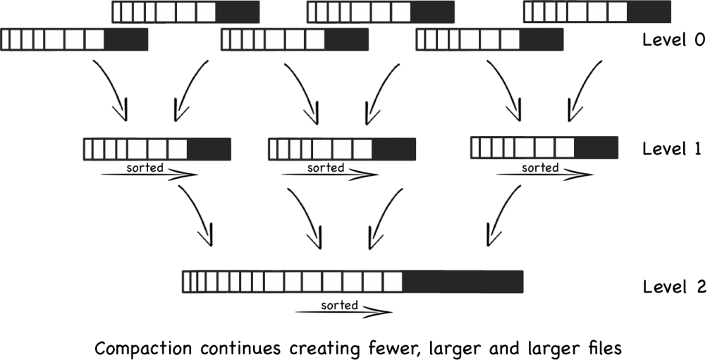
When a certain number of files have been created, say five files, each with 10 rows, they are merged into a single file, with 50 rows (or maybe slightly less) .
This process continues with more 10 row files being created. These are merged into 50 row files every time the fifth file fills up.
Eventually there are five 50 row files. At this point the five 50 row files are merged into one 250 row file. The process continues creating larger and larger files. See fig.
The aforementioned issue with this general approach is the large number of files that are created: all must be searched, individually, to read a result (at least in the worst case).
Levelled Compaction
Newer implementations, such as those in LevelDB, RocksDB and Cassandra, address this problem by implementing a level-based, rather than size-based, approach to compaction. This reduces the number of files that must be consulted for the worst case read, as well as reducing the relative impact of a single compaction.
This level-based approach has two key differences compared to the base approach above:
1. Each level can contain a number of files and is guaranteed, as a whole, to not have overlapping keys within it. That is to say the keys are partitioned across the available files. Thus to find a key in a certain level only one file needs to be consulted.
The first level is a special case where the above property does not hold. Keys can span multiple files.
2. Files are merged into upper levels one file at a time. As a level fills, a single file is plucked from it and merged into the level above creating space for more data to be added. This is slightly different to the base-approach where several similarly sized files are merged into a single, larger one.
These changes mean the level-based approach spreads the impact of compaction over time as well as requiring less total space. It also has better read performance. However the total IO is higher for most workloads meaning some of the simpler write-oriented workloads will not see benefit.
Summarising
So LSM trees sit in the middle-ground between a journal/log file and a traditional single-fixed-index such as a B+ tree or Hash index. They provide a mechanism for managing a set of smaller, individual index files.
By managing a group of indexes, rather than a single one, the LSM method trades the expensive random IO associated with update-in-place in B+ or Hash indexes for fast, sequential IO.
The price being paid is that reads have to address a large number of index files rather than just the one. Also there is additional IO cost for compaction.
If that’s still a little murky there are some other good descriptions here and here.
Thoughts on the LSM approach
So are LSM approaches really better than traditional single-tree based ones?
We’ve seen that LSM’s have better write performance albeit a cost. LSM has some other benefits though. The SSTables (the sorted files) a LSM tree creates are immutable. This makes the locking semantics over them much simpler. Generally the only resource that is contended is the memtable. This is in contrast to singular trees which require elaborate locking mechanisms to manage changes at different levels.
So ultimately the question is likely to be about how write-oriented expected workloads are. If you care about write performance the savings LSM gives are likely to be a big deal. The big internet companies seem pretty settled on this subject. Yahoo, for example, reports a steady progression from read-heavy to read-write workloads, driven largely by the increased ingestion of event logs and mobile data. Many traditional database products still seem to favour more read-optimised file structures though.
As with Log Structured file systems [see footnote] the key argument stems from the increasing availability of memory. With more memory available reads are naturally optimised through large file caches provided by the operating system. Write performance (which memory doesn’t improve with more) thus becomes the dominant concern. So put another way, hardware advances are doing more for read performance than they are for writes. Thus it makes sense to select a write-optimised file structure.
Certainly LSM implementations such as LevelDB and Cassandra regularly provide better write performance than single-tree based approaches (here and here respectively).
Beyond Levelled LSM
There has been a fair bit of further work building on the LSM approach. Yahoo developed a system called Pnuts which combines LSM with B trees and demonstrates better performance. I haven’t seen openly available implementations of this algorithm though. IBM and Google have done more recent work in a similar vein, albeit via a different path. There are also related approaches which have similar properties but retain an overarching structure. These include Fractal Trees and Stratified Trees.
This is of course just one alternative. Databases utilise a huge range of subtly different options. An increasing number of databases offer pluggable engines for different workloads. Parquet is a popular alternative for HDFS and pushes in pretty much the opposite direction (aggregation performance via a columnar format). MySQL has a storage abstraction which is pluggable with a number of different engines such as Toku‘s fractal tree based index. This is also available for MongoDB. Mongo 3.0 includes the Wired Tiger engine which provides both B+ & LSM approaches along with the legacy engine. Many relational databases have configurable index structures that utilise different file organisations.
It’s also worth considering the hardware being used. Expensive solid state disks, like FusionIO, have better random write performance. This suits update-in-place approaches. Cheaper SSDs and mechanical drives are better suited to LSM. LSM’s avoid the small random access patters that thrash SSDs into oblivion**.
LSM is not without it critics though. It’s biggest problem, like GC, is the collection phases and the effect they have on precious IO. There is an interesting discussion of some of these on this hacker news thread.
So if you’re looking at data products, be it BDB vs. LevelDb, Cassandra vs. MongoDb you may tie some proportion of their relative performance back to the file structures they use. Measurements appear to back this philosophy. Certainly it’s worth being aware of the performance tradeoffs being selected by the systems you use.
**In SSDs each write incurs a clear-rewrite cycle for a whole 512K block. Thus small writes can induce a disproportionate amount of churn on the drive. With fixed limits on block rewrites this can significantly affect their life.
Further Reading
- There is a nice introductory post here.
- The LSM description in this paper is great and it also discusses interesting extensions.
- These three posts provide a holistic coverage of the algorithm: here, here and here.
- The original Log Structured Merge Tree paper here. It is a little hard to follow in my opinion.
- The Big Table paper here is excellent.
- LSM vs Fractal Trees on High Scalability.
- Recent work on Diff-Index which builds on the LSM concept.
- Jay on SSDs and the benefits of LSM
- Interesting discussion on hackernews regarding index structures.
Footnote on log structured file systems
Other than the name, and a focus on write throughput, there isn’t that much relation between LSM and log structured file systems as far as I can see.
Regular filesystems used today tend to be ‘Journaling’, for example ext3, ext4, HFS etc are tree-based approaches. A fixed height tree of inodes represent the directory structure and a journal is used to protect against failure conditions. In these implementations the journal is logical, meaning it only internal metadata will be journaled. This is for performance reasons.
Log structured file systems are widely used on flash media as they have less write amplification. They are getting more press too as file caching starts to dominate read workloads in more general situations and write performance is becoming more critical.
In log structured file systems data is written only once, directly to a journal which is represented as a chronologically advancing buffer. The buffer is garbage collected periodically to remove redundant writes. Like LSM’s the log structured file system will write faster, but read slower than its dual-writing, tree based counterpart. Again this is acceptable where there is lots of RAM available to feed the file cache or the media doesn’t deal well with update in place, as is the case with flash.
Building a Career in Technology
Friday, January 2nd, 2015
I was asked to talk to some young technologists about about their career path in technology. These are my notes which wander somewhat between career and general advice.
- Don’t assume progress means a career into management – unless you really love management. If you do, great, do that. You’ll get paid well, but it will come with downsides too. Focus on what you enjoy.
- Don’t confuse management with autonomy or power, it alone will give you neither. If you work in a company, you will always have a boss. The value you provide to the company gives you autonomy. Power comes mostly from the respect others have for you. Leadership and management are not synonymous. Be valuable by doing things that you love.
- Practice communicating your ideas. Blog, convince friends, colleagues, use github, whatever. If you want to change things you need to communicate your ideas, finding ways to reach your different audiences. If you spot something that seems wrong, try to change it by both communicating and by doing.
- Sometimes things don’t come off the way you expect. Normally there is something good in there anyway. This is ok.
- The T-shaped people idea from the Valve handbook is a good way to think about your personal development. Have a specialty, but don’t be monomaniacal. What’s your heavy weaponry?
- Whatever speciality you find yourself in, start by really knowing the fundamentals. Dig deep sooner rather than later as knowledge compounds.
- Always have a side project bubbling along. Something that’s not directly part of your job. Go to a hack night, learn a new language, teach yourself to paint, whatever, it doesn’t need to be vocational, just something that broadens your horizons and keeps you learning.
- If you find yourself thinking any particular technology is the best thing since sliced bread, and it’s somewhere near a top of the Gartner hype-curve, you are probably not seeing the full picture yet. Be critical of your own opinions and look for bias in yourself.
- Pick projects that where you have some implicit physical or tactical advantage over the competition. Don’t assume that you will do a better job just because you are smarter.
- In my experience the most telling characteristic of a good company is that its employee’s assume their colleagues are smart people, implicitly trusting their opinions and capabilities until explicitly proven otherwise. If the modus operandi of a company (or worse, a team) is ‘everyone else is an idiot’ look elsewhere.
- If you’re motivated to do something, try to capitalise on that motivation there and then and enjoy the productivity that comes with it. Motivation is your most precious commodity.
- If you find yourself supervising people, always think of their success as your success and work to maximise that. Smart people don’t need to be controlled, they need to be enabled.
- Learn to control your reaction to negative situations. The term ‘well-adjusted’ means exactly that. It’s not an innate skill. Start with email. Never press send if you feel angry or slighted. In tricky situations stick purely to facts and remove all subjective or emotional content. Let the tricky situation diffuse organically. Doing this face to face takes more practice as you need to notice the onset of stress and then cage your reaction, but the rules are the same (stick to facts, avoid emotional language, let it diffuse).
- If you offend someone always apologies. Always. Even if you are right, it is unlikely your intention was to offend.
- Recognise the difference between being politically right and emotionally right. As humans we’re great at creating plausible rationalisations and justifications for our actions, both to ourselves and others. Making such rationalisations is often a ‘sign’ of us covering an emotional mistake. Learn to notice these signs in yourself. Look past them to your moral compass.
A World of Chinese Whispers
Thursday, May 1st, 2014
For the summary: TL;DR
It may seem surprising but the seemingly benign and somewhat soporific subject of “data movement” turns out to be a contentious and well scrutinised problem in many large organisations. There’s good reason for this. With the best will in the world, when you have two systems using the same data, getting them to stay in sync over time is really hard. When you have a web of interconnected systems sharing data it’s even harder. When you’re talking about historic state it’s harder still. In fact it’s one of the toughest classes of problems known to software engineering, involving lots of people, different systems, impedance mismatches at a data level and worst of all; really really slow feedback loops. Problems like this make NP hard look like a short afternoon of intellectual flirting. This problem is BFS Hard. Big and F-ing Slow Hard!
But it’s also really important. Businesses are faced with embarrassing situations where figures don’t match, arguments ensue, regulators get stroppy, armies of project managers and analysts turn up, you get the picture.
Many organisations pin their hopes on messaging, usually kept in check by a schema controlled by some central architecture group. This is a sensible step away from point to point file transfer; a notoriously problematic set up akin to a game of Chinese whispers but with a common tongue that isn’t native to anyone. Despite many benefits however, unified messaging is not without its own problems.
If we look a little deeper we find two specific issues. The first is that systems transform both ‘onto’ and ‘off’ the wire. Two distinct points of bespoke transformation. Two opportunities for things to diverge from the truth.
The second problem is that maintainer of the data, usually the source, is rarely good at propagating historic changes they make, locally. More divergence occurs over time.
In fairness this isn’t a problem for very simple, static data structures. But it becomes increasingly complex for broarder schemas and particularly statefull entities (one’s that change state in complex ways over time).
One common response is some form of Enterprise Data Warehouse (EDW) that collects all the company’s state. The EDW pattern also suffers as it has to maintain the full complexity of a centralised schema, and all the work to translate into it. It is also subject to the quality of the data it receives. For many EDWs the inbound data is pretty deficient because it’s produced at source as an after affect.
EDW’s do work though. Many companies have implemented them with success. But they are another BFS hard problem: slow, arduous and expensive.
More recently data lakes push the problem of schematic conformity to the point of consumption. This is a good idea, but there is more we can do.
The nirvana though, at least in my opinion, is a synergy between the system of record (used to hold history), the wire format used for streaming use cases, and a set of mirrored copies used around the organisation, each of which provides freedom for bespoke queries and data processing.
Before we get to that though lets look at different approaches used to date to distribute information through a company.
One Central Copy or Distribute Everywhere
The problem we are trying to solve, ultimately, is a simple one. Teams want a range of data, which is authored elsewhere, either as a realtime stream, or via a database, so they can run business processes and hopefully make some money for the shareholders.
The simplest blank-canvas approach would be have a single all-singing-all-dancing database that everyone both wrote to and read from. This would ensure that all state existed only once, it would be consistent, by definition, and would be available to all. Awesome!
But such an organisation would look more like a mainframe of days of old. I’ve joked about this before. Such a seemingly abhorrent analogy may be unwise, but it does force focus on the pros and cons of the situation we find ourselves in, so bear with me for a moment.
 The mainframe’s benefits are (a) it stores state just the once, and in a single form and (b) it’s easily accessible by all the services in the mainframe.
In most companies we, on the other hand, store state in many places, in many forms.
But the mainframe pattern doesn’t scale very well. Not so much from a performance perspective, although that is a valid concern, but rather it is operationally limited. Its inability to change and adapt quickly to the varied needs of a company make it a hard pattern to use on a macroscopic level.
It is the same failure we might pose to an enterprise that tried to coordinate itself around a single database. It would fall into an immobile lock-step world in which no one would get anything done. Because the pattern is implicitly restrictive and teams would end up creating data marts and the like just to get things done. This problem is prohibitive, or at least it may seem to be.
Many internet companies, who grew quickly around a common goal, are arranged around shared datastores. Ebay use Teradata, Google have their own database. Amazon’s is based on their internal platform services which they now expose to others (Dynamo, S3 etc). In fairness they all have a fair bit of fragmentation too, but they are in better shape than many traditional enterprises.
The difference is that, in these companies, making your data available to someone else is comparably straight forward. That’s to say it’s easier to go straight to the source where all the history is. This is one thing the enterprise needs to change. Enterprises generally keep their data in relational databases and are scared to expose this state to others, for fear of the performance and management issues that would result.
What we want is a world where originating sources can focus on data content, not on distribution. Infrastructure should make sharing state easy, both as a stream and as a historic query or mirror.
 Enterprises have, for some years, gone the other way. Messaging is used to shift data from system to system. This promotes decoupling. It also provides a lingua franca if a central schema is imposed. This helps companies discuss the meaning of their data and relate concepts across systems.
The cons are that the lingua franca generally only exists for that small time the data is on the wire. It is rarely written down this way.
This limits the benefit simply because it is so short lived. Both source and destination will likely have their own schema and often look quite different from one another. Transformation, because it is generally handcrafted, is buggy.
The tenet this leads to is this:
Messaging should be used to allow applications to act, to kick off processing, to notify a user, to *DO* something. It should not be used for the bulk transfer of (historically held) state between databases.
A Middle Ground: Data Virtualisation?
One solution often touted by integration companies is Data Virtualisation*. This pattern has been implemented in large organisations with some success. Data is left where it is, with the history intact. This reduces the probability of divergence.
* Data virtualisation is a layer that sits over a set of databases and provides an aggregate view either via union, or more usually join. Predicates are pushed down to the underlying databases and joined as the query from each database returns.
Data Virtualisation has failings too though. The first is operational. Testing requires that the different, independent sources be aligned so that the data joins up. This is hard to do in practice because it requires fine grained cross-team coordination. Not insurmountable, but hard. Maybe even BFS hard.
The second problem is performance where data has to be joined across systems rather than performing a union. Use cases which work best have only one large dataset and queries focus on retrieval rather than aggregation (*1).

The final problem is more ideological. It’s tempting to place Data Virtualisation on an architecture diagram and funnel everything through it. This is the ‘Silver Bullet’ syndrome.
In reality we need to be mindful of the above shortcomings and have solutions that counter-balance. Only with this can the pattern succeed.
Data Virtualisation upholds the basic premise that, if we value accuracy, data is best left where it is authored.
But the value of the data virtualisation approach is that it upholds the basic premise that, if we value accuracy, data is best left where it is authored. As such data virtualisation can be a good first step in an integration architecture, for reporting (set-based) use cases. But my fear is that many companies will continue to struggle with the operational issues that come with it.
The Inevitable Collocation of Data
So, whilst Data Virtualisation is well suited to many use cases, data will need to be moved one way or the other for more arduous joins and bespoke processing. It also makes sense to replicate this state using the same schema that the Data Virtualisation layer uses. That’s to say; the one used by the source. Enterprise Messaging isn’t a great fit for this kind of bulk data collocation simply because it drags the data away from the source’s persistence format, so the best option is to simply mirror the source data using a a log streaming technology.
The advantage of mirroring is that data is materialised with the full history intact. Being a ‘binary’ replica this is analogous to having the golden source data directly on hand. Changes to the source dataset are communicated without translation. It’s an exact, and ongoing, clone.

Cloning databases is not a new idea, people have been creating mirrors for literally decades and there is mature relational technology in this space. However there is less evidence of its use for large-scale data integration. Certainly the implications of following such an approach are not trivial, if an only because the result is more tightly coupled.
What has changed in recent times is NoSQL technology provides richer semantics for replication. Many NoSQL products can provide both synchronous read-replicas and asynchronous clones off the shelf. This provides powerful low level metaphors for composing solutions.
There are also now a wealth of open source tools that can help with this kind of architecture. Technologies like Tungsten provide interfaces to write ahead logs. This turns source databases into data streams. Tools like Kafka can handle the throughput levels of many concurrent streams of this type. Data can be collected in other relational databases, simply as mirrors. Placed into a data lake and processed with Hadoop based tools or streamed to applications for direct processing. The key point is to make data available without translation to any centralised format. If the source format sucks, fix it!
There are some big advantages to this approach: you don’t have to write feed code just to get access to data. We should be able to simply materialise it where it is needed. Secondly the pattern is faster to implement than Messaging + EDW because it is federated. The EDW concept can just be a single consolidation point.
There are however a number of problems to overcome. It must not be brittle, it must not require lock-step releases and consumers must not be unduly affected by maintenance activities going on in golden sources.
This would mean a number of changes would need to be made. The role of being a golden source would be more arduous. Rather than simply taking responsibility for sending messages, they are responsible for maintaining a historic data set which is replicated to ’n’ different production stores. In particular, in the relational world, a small tweak at source can result in significant data transfers. This is why the infrastructure and governance needs to be good.
Sources would also need to uphold some fairly stringent rules because there is less opportunity to fix things up during the traditional ETL phase (*2).
So in summary, if you want some data, go to the source. If the source worries about its performance, create a mirror. If you want to react to a stream, listen to the one that keeps the mirror up to date. If you need to do completely your own thing, take a mirror for yourself and off you go. But make sure the mirror is an exact ‘binary’ replica of the source, not a feed that has been ETL’d, or a flat file or any other cooky mechanism held together with string, good will and a smattering of enterprise architects.
The Duality of Database and Stream
Most sensible database users implement a bitemporal model. This is a model that stores all changes as versioned data. Other designs include audit tables. Suffice to say that it’s pretty well accepted that journalling state-changes is a good idea.
What is an event stream or log? It’s a journal of state changes. A large system I helped build used messaging as the system of record, simply because making your system of record a stream makes it very easy to materialise that stream in different types of databases in different locations.
So are databases and messaging systems related? Jim Gray, of Microsoft Research, believed all queues were databases. With functionality like message selectors (which is essentially a query) there is a strong relationship between them. On the other hand the disk organisation is generally very different.
What I find inevitable is that both services will be provided by the same infrastructure. The reasoning for this is clear. There is much to be gained from listening to state and correlating that with other data, from the same point in time, as we query.
Looking to the Future

The enterprise of the future will look different. We won’t think of many of these problems. A project might start with a self-service console that provisions a persistent environment with whatever data they need, magically kept up to date for them, or alternatively an equivalent stream. Snapshots and release windows will make coupling manageable. The whole thing will be a service that is provided by the infrastructure.
So this is no mainframe, it is not a single organisational database or warehouse. It is best thought of as a collection of independent databases, which appear autonomous to their users, but with inbuilt data provisioning and greater storage and performance potential than we are used to today. This would be provided through an interlinked ‘backbone’. The backbone moves data between different machines to provide both scaling, data locality and predictable performance.
So this is not a campaign against enterprise messaging, instead it is a campaign for changing what it is. What we need is a synergy between event state and persisted state. They need to be but two sides of the same coin. The authoritative stream of state for some fact is the same as the chronological table scan for that fact.
The future sits with integration technology that provides symmetry between data in motion and data at rest so that scaling read access to data, at a company level, is simply a function of the infrastructure.
TL;DR
This article campaigns for a change to what enterprise messaging and even data warehouses are. Companies need infrastructure that provides a synergy between event state and persisted state. They need to be two sides of the same coin.
The authoritative stream of state for some fact should be exactly equivalent to the lowest level, chronological table scan for that same fact. This provides a symmetry between this data in motion and data at rest.
The result is reads that scale automatically through infrastructure. This removes the key boundaries that stop us sharing data at source.
Key points:
- Messaging the need to act on something works well. Notifying that a trade was booked results in an action to kick off the settlement process. But too much focus on a centralised schema can be counter productive. Real systems with complicated data models have to put great effort into translating both ‘into’ and ‘out of’ the “Enterprise Data Model” used on the wire. As time passes and data ages the different copies get more and more out of sync.
- The approach pushes us down a path of ETL on both sides of the wire. So simple problems like: I need a list of customers become hard problems. You have to build a feed, running a feed processor, persist the data and keep it accurate over time. Where relational databases are used this is non-trivial.
- ‘Mirroring’ state from persistent form to persistent form via a streaming layer is a better option. Think of this a large scale database replication if you prefer. It’s better because it favours accuracy, albeit at the price of tighter coupling.
- Managing this tighter coupling offers challenges, but is within our means. Data Virtualisation can be used as stepping stone in some cases. Data streaming (mirroring) is the more general (if more heavyweight) solution.
- We need the wire data model and the persistent data model to match.
- BigData and open source technologies provision for this. They provide the infrastructure needed to build out this kind of solution: Tungsten, HDFS, Cassandra, Mongo, Kafka etc. It can be solved relationally too, just in different ways. The key is that event and persisted state are two sides of the same coin.
- Finally publishers need to be well behaved. This pattern pushes responsibility to them to provide good quality data. Fixing at source avoids some of the sluggishness seen in many Enterprise Data Warehouse implementations, but it does require significant sponsorship to get sources to behave well.
Footnotes:
(*1) The golden sources would also need to adhere to some fairly stringent rules. Most notably the view presented to consumers should:
- Provide an immutable (versioned) history of changes, with a marker that defines the most current version.
- Provide a bi-temporal view, so that data can be viewed in terms of wall-clock and business times (wall-clock time must be consistently stamped as the system clock is required to ensure read consistency across async copies)
- Guaranteed backward compatibility of a published view (that is to say that tables and columns may be added but not changed or removed).
- A rolling set of two (or three views) to allow consumers to adopt non-backwardly compatible changes (where tables or columns have changed or been removed) without requiring a lockstep release.
- Any changes to these externally accessible views would need to be scheduled to ensure they do not put undue load on consuming systems.
(*2) The distributed optimiser, found in Data Virtualisation products, has relatively few options when faced with a query that joins two large datasets. It can query both sides, ordering by the join-key, and perform a merge-join. It can query one side of the join and dip into the other via in(key, key, key…), it can further optimise by bringing the second key-set, or entire recordset, into the virtualisation layer upfront.
These techniques become problematic where two large datasets are combined and inner-joins significantly clip the result set. Aggregations, which span both sides of the join condition, suffer from a similar problem. Both of these require the movement of a significant amount of data into the virtualisation layer, for a comparably smaller result. This makes them slow.
References:
- There are a number of open source tools including Escada, Symmetricds and slony-I.
- There is a good comparison of these vs commercial products here.
- A financial use case here
Database Y
Friday, November 22nd, 2013
MongoDB recently secured $150m in funding. If you’re not sure how to place that figure, it is more than any database vendor has secured in a single funding round, ever! The company was reportedly valued at $1.2 billion, a huge amount considering the total annual revenue in the NoSQL market was only $542m in 2012. News reports of new databases appear on what feels like a weekly basis. The latest database landscape cites more than two hundred products, and only really scratches the surface.

So this is an interesting time for the database world and there are some inevitable questions arising from where these change have come from. Certainly it would seem that the database field has not been serving us, the customers, sufficiently well. If it were these new products would be unlikely to exist. Behind this likely sits a more fundamental change in our needs. The internet has been an obvious contributory factor but there is likely more to this change than simply the need to scale. Joe Hellerstein, something of a guru in the database field, called this out more than a decade ago, and his words make interesting reading today with provocative, if informal, comments like:
“Databases are commoditized and cornered … to slow-moving, evolving, structure-intensive apps that require schema evolution”
The 90s classic The Innovators Dilemma also resonates. In it Christensen describes a cycle of replacement, arising from the blinkered following of customer’s contemporaneous needs.
The companies that innovate, in the Christiansen sense, tend to operate in smaller, niche markets that are less well served; markets that tolerate the rough edges that new products inevitably have. These innovations often pre-empt changes in the mainstream. If and when shifts occur the mainstream incumbents can be left lacking the expertise they need to compete.
Amongst other examples he cites analysis of hard disk production in the 80s where Seagate came to dominate the hard disk market when it shifted from 8” to the smaller 5.25” format. The manufactures of the larger 8″ format missed a trick. Preoccupied with increasing the performance of the 8” format, preferred by mainframe customers, they could not complete when the market changed. They had listened to their customers, and followed the most profitable of sales, but in doing so they missed what, in hindsight, seems like an obvious shift , but likely seemed less clear cut at the time.
As computers got smaller. Seagate, having cut their teeth in 5.25” technology for the best part of a decade selling to the then niche desktop computer market, cleaned up.
So I find myself wondering if the database world with its flourishing, open source wedded NoSQL movement may be following this pattern?
Whist it seems unlikely that the latest bedroom-crafted distributed hash table will oust the likes of Microsoft, Oracle and IBM that does not mean that the pattern will not play out in one form or other. Enterprise customers are not demanding change in the same way the internet companies are and with enterprise customers making up the lion’s share of the database gravy train the money is not going anywhere fast. The interesting question is whether there is something genuinely disruptive here? Something that could leave the incumbent database vendors lacking.
One of the key problems that many of the NoSQL (and NewSQL) vendors face is the absence of the rigorous heritage of the traditional database products. Databases are complicated software, the most complex libraries you will likely program with on a day-to-day basis. Most recent relational database contenders; Aster Data, ParAccel, Greenplum, Netezza, Vertica – to name just a few of many – have been Postgres forks. This being necessary to get a leg up the steep development curve required to build a fully functional DBMS.

NoSQLs; Couchbase, Cassandra and Dynamo (Voldemort) are all under 200k lines of code, a questionable metric I know, but it hints to the comparative simplicity of some of these solutions.
The NoSQLs are, in many ways, slightly crappy products. A quick scour of the Internet will find you numerous articles citing the crappyness of Mongodb. It’s strange and weird failure scenarios, overly simplistic delegation of IO to the operating system and (the now changed) default policy to not put any of your data on disk synchronously. The MongoDB is Webscale clip plays on this to hilarious ends.
Yet the market is surprisingly tolerant, at least for the meanwhile. The Christiensen explanation would be that niche markets are inherently tolerant of slightly crappy products because there is simply less to compare them to. The first Walkman, personal computer, mobile phone were all actually pretty crappy. They were however also very cool. They did stuff that the mainstream did not, opening markets that were previously unavailable. Few large corporates manage to do this (Job’s Apple being the obvious counter).
Despite being a little rough round the edges, the use of Mongo has gone viral . The recent valuation of 1.2 billion evidences this success. Marklogic, a far more mature, solid (and expensive) NoSQL with a heritage in XML document storage, makes for an interesting comparison. Marklogic has also had commercial success (Wikibon putting Marklogic as the dominant player in the NoSQL space – see graphic) but has nothing like the community penetration of Mongo. Google Trends puts this well (lower graphic) and VC money in this day and age often follows the horde rather than the balance sheet.
Part of this success can be attributed to the open-source pricing model. Open source makes technology more accessible, coming in under the corporate radar. People are more tolerant of something that is free. Finally and importantly it has a laid back dressing of web-cool that captivates young engineering minds… although that might change if a Oracle-esque corporate sales machine kicks in.
So if NoSQL is simply about scaling then why Mongo’s recent success? Mongo has a fraction of the scalability of Aerospike, Riak or Dynamo. This is because it has chosen the less scalable, but far more user friendly free-form query API which puts it far closer to the traditional OLTP space than other products in the NoSQL space.
Possibly more importantly it panders to the iterative, poly-structured world of today’s engineers and in doing so it is locking into a fundamental truth: the relational world doesn’t sit well with today’s development practices and the latest generation of programmers are less wedded to it than the last.
So are we witnessing an interesting niche field growing up or is this the prologue for a Christiensen-style shift of the mainstream?
Oracle took $11 billion of the $34 billion database market in 2012. The whole NoSQL market is a little over half a billion currently (2%), so it seems unlikely that Larry will be quaking in his platinum-coated deck shoes just yet. But to Christensen’s point, if the differentiation is both significant and sustained and the mainstream vendors do not keep up, that could spell change.
It is unclear to me, as it stands today, whether this path is really disruptive. I’ve discussed the signs of convergence before but there are also a number of technical approaches that are acting as differentiators: The use of shards and replicas are in many ways more advanced that those seen in relational systems. The application of schema on need provides an iterative, explorative approach to data-modelling and data-model evolution. More progressively No/NewSQL is moving beyond CAP to include lightweight transactional models that provide stronger consistency guarantees without all the baggage of serialisable two-phase commit.

So whether this is tangential or revolutionary remains to be seen. Intuitively it certainly seems unlikely that David will topple any of the Goliaths, in fact it seems more likely that the Goliaths with simply eat (buy) the Davids, but we should still see deeper changes than those evidenced by the current lip service paid by the big vendors. This is a good thing.
Big Data’s ill-defined promise of otherwise missed insight has done more for bolstering vendor sales figures than it has to derive value in many of the organisations that implement it.
That’s not to say that it is without successes, far from it. Empirical exploration of customer behaviours has changed the way we interact with customers and has in fact raised the bar for all online custom. But approaches like bolting a MR framework onto to an existing storage engine or adding a JSON column type smack more of feature-sheet bolstering then they do of true technical innovation.
Instead the big vendors should look to the world of today’s engineers: cheap commodity hardware, agile development, continuous integration / delivery, poly-structured data both on the wire and in programs and a general lack of tolerance for anything that removes control from the development process. Mongo’s success can certainly be attributed, at least in part, to this.
The relational world is however both deeply embedded and wholly trusted, and so it should be. Data is something that lasts for decades and holding long-lived data in a schemaless store will bring with it many additional challenges not seen today. This fact alone may see truly schemaless stores marginalised in the long run.
But the generational thing may be decisive. If decision makers in large companies have one thing in common it is their age. Having sat through decades of relational dominance we can cite a thousand sensible, logical, often unquestionable reasons why this dominance should continue. Generation Y however are simply less likely to see it the same way.
The Big Data Conundrum
Saturday, November 10th, 2012
I attended an interesting talk at JAX earlier this year by guy called Ian Plosker, from Riak, somewhat amusingly entitled ‘TheBigDataCon’ (worth a look by the way – the slides are good). Ian makes a little fun of all the current hype, joking that vendors seemed to be the only people actually monitising Big Data. I think we can’t help but be a little cynical of anything that has this much hype.
On another level the term has become overloaded. It has many definitions, Oracle for example talk about Big Data in a very different way to say MapR. It seems to broadly boil down to two angles though:
- The promise of greater insight using the huge amounts of data we produce
- A change in the technologies we use to crunch our way through the data we have (or expect to have)
Like any other commodity, the harder it is to extract, the more it costs. The aspirational, needle-in-a-haystack concept that drives much of the marketing paraphernalia is certainly real and should not be ignored. However the hype around the ‘hidden insight’ thing masks a more fundamental, and grounded point: the technology shift that facilitates all this.
There is a view that todays data is ‘big’ and that having big data means some form of MapReduce. Yet it is not size that really matters. Both relational and nosql camps can deal with the data volumes (and even, for the most part, the three Vs in one way or another). Ebay for example runs a 20PB+ database. Yahoo and Google both have larger MR clusters, but not that much larger. For most problems data volume alone is not enough to make a sensible technology choice (and I’d contest that any of the Vs were really enough either). As the academic world likes to keep reminding us (here and here) performance is not the reason to pick up a big data technology. There reason is that these new technologies embrace a very different approach to data analysis, particularly in the context of the whole ‘lifecycle’ of our data analysis work. Big Data technologies decouple us from some of the shackles that make big data problems hard. However, there is no free lunch and they come with some shackles of their own.
A core difference is the ability to define a schema at runtime, rather than upfront. That alone is a powerful, and game changing idea. Dave Campell put it well in his VLDB keynote when he says ‘ability to model data is much more of a gating factor than raw size, particularly when considering new forms of data’. Modelling data, getting it into a form we can interpret and understand can be a longwinded and painful task, and something we must do before we can do anything useful with it.
Our ability to model data is much more of a gating factor than raw size
Traditional databases push us to model our data before we store it. Big data solutions often leave their data in its natural form. A ‘virtual schema’ is bound at runtime. This concept of binding the schema ‘late’ is powerful. It allows the interpretation of the data to be changed at any time without having to change the physical format of the data on disk. Something that becomes increasingly important as the size of the dataset increases. The downside of not imposing a schema from the point of ingestion is that keeping old forms of data ‘current’ becomes an increasingly difficult task. That’s to say that the client is left with the problem of handling many data representations. Fine if the model is free text, tougher if the model has any real structure (explicit or implicit).
The concept of binding the schema ‘late’, with the data held in its natural form, is powerful.
Big Data technologies offer very different performance profiles to relational analytics tools. The lack of indexing and overarching structure means inserts are fast, making them suitable for high velocity systems and batch processing. The imperative interface and the absence of a schema, makes diverse, ad hoc analytics hard though. Instead they work best for specific, well-defined data operations (I often use the data enabled grid analogy). It is likely this that has driven Big Data leaders, Google, and more recently Hadoop, to add more database-like features to their products (Dremel/Magastore/Spanner providing SQL like interface and ACID semantics). Yet it’s much harder to optimise in a late-bound world, no big data solution today comes close to the raw performance of the top end analytics engines.
Most of today’s databases are hindered hugely by needing the schema to be defined upfront.
The last thing to consider is the cost of change. For simple data sets it is less apparent. Start joining data sets together though and it becomes a different ball game. Whist possible with Big Data technologies, it’s just going to cost more and managing the complexity with the absence of a schema becomes an increasingly uphill struggle. In this case, better to stick in the relational world (for now at least).
However most of today’s databases have the HUGE disadvantage that the schema needs to be defined, and the data understood, upfront. Great for simple, well defined business data, but if you’re searching free text, machine generated data or simply a hugely diverse data population (like the data that gets thrown around most big organisations) it’s simply not practical or maybe not possible to understand, and model, the data upfront. By applying the schema later in the cycle the cost of change, the availability of insight and the inherent feedback cycles can all be improved.

As for the future?
You’ll probably have noticed that every database vendor worth their salt now have some form or Big Data offering, be it bought in, ‘tacked on’ or genuinely integrated. Likewise the Big Data vendors are looking more and more like their relational counterparts, sprouting query languages, loose schemas, columnar storage, indexing, even elements of transactionality. The two camps are converging.
Many of new set of relational technologies look more like MapReduce than they do like System R (IBM’s original relational database). Yet the majority of the database community still seem to be lurking in the corner of the playground, wearing anoraks and murmuring (although these days the anoraks are made by Armani). They are a long way from penetrating the progressive Internet space. Joe Hellerstien’s words still ring true today.
The new cool kids of the database world are making their mark with technologies of the moment, backed with a hefty dose of academic acumen.
The future is likely to be one of convergence, and redirecting the database community is undoubtedly good. In fact possibly the most most useful things the NoSQL movement has done has been to give a well timed boot to the database world’s behind, reminding them that they need to listen to their consumers. They got stuck in a rut and the internet space wasn’t going to wait around. Convergence over some newly shared values that sit between the two camps is of course inevitable, and welcomed.
The database world got stuck in it’s ways and the internet space wasn’t going to wait around.
The evidence is quite plain already. There are a host of young (ish) upstart technologies hitting the space. The number of shared nothing analytics engines has significantly increased (Asterdata, Vertica, VoltDB, Exasol, ParAccel, Greenplum, Hana the list goes on) and the benchmarks they are extremely impressive. There are hybrid engines mixing MapReduce engines with smarter storage, routing and indexing strategies. Hadapt and Impala are good examples. The former particularly as it is the one that probably best personifies the blending of the two worlds.
These new upstart database technologies redefine the current mainstream with, not in spite of, the lessons of the past.
Finally there are some interesting one-stop-shop approaches. Holistic solutions that span dynamic schema provisioning and data access, all the way to presentation in a single package. Originating in the machine generated data space, Splunk (dominant) and Logscape (scalable), are the current leaders in this space and there is likely to be a lot more activity. For answering the what-if questions or assembling high level MI stacks these all inclusive solutions get the closest to answering the more insightful questions we have today.
Whether this ever breaks the strangle hold clenched by the oligopoly of key database players remains to be seen. Michael Stonebraker still rains disdain on the NoSQL world even today [see here]. He may be outspoken, he may come across like a bit of **** at times, but it is unlikely that he is wrong. The solutions of the future will not be the pure (and relatively simplistic) MapReduce of today. They will be blends that protect our data, even at scale. For me the new technologies coming from both camps are exciting as they redefine the current mainstream thinking with, not in spite of, the lessons of the past.
Related posts:
Where does Big Data meet Big Database?
Saturday, July 28th, 2012
[This post is adapted from a QCon talk I gave in 2012: Where Big Data meets Big Database]
Databases are amazing technology. Despite sitting on clunky, highly sequential media, they remain spriteful and reactive to a whole range of random user requests.
Yet a community that was once the height of technological innovation appears to have sat on its laurels somewhat in recent years. Lucrative support contracts, from a mass of corporate dependents, no doubt further this sense of apathy.
NoSQL and the Big Data upstarts, hungry for a piece of the pie, appear fresh and vibrant, blowing a breath of fresh air into the cobwebbed world of rows and columns. Whilst still inferior in many ways they have forced a rethink of how data should be stored, accessed and processed. This is a good thing.
But the marketing surge that has come with it is something of a mixed blessing. You can barely move for the hype. There are also many misconceptions, particularly around the technology itself. One of the most notable is the misconception that handling large data sets necessitates something that looks like Hadoop. At the other end of the spectrum the ‘big three’ database vendors are touting products that look very much like the products of ten years ago. Big Data seems to have caught them off guard and they seem to be floundering somewhat, pinning Big Data emblems to their existing products without really rethinking their approach to problem in the context of today’s world.

This apparent apathy is highlighted by the host of upstart database and NoSQL technologies that have achieved market penetration. The database market is not an easy one to get into. It is an oligopoly, in economic terms: A market dominated by a small number of key players. The barrier to entry is high, making it hard for smaller companies to penetrate. The products are similar, largely interchangeable and no one vendor has total monopolistic control. In fact many markets end up in this state. Mobile technology and service provision, oil, airlines etc. The database industry is one of these too and has been for twenty years. Yet there are today something in the order of two hundred viable vendors in different segments. A smaller group of these fledgling brands have gained real traction. The implication being that the mainstream must be missing a trick somewhere, at least it’s not fully catering to its customer’s needs.
Their ‘way in’ has been products that pander to subtly different use-cases. Some sold as databases, some NoSQL stores, some BigData. The categories are starting to blur but the general theme favours simpler contracts to achieve scalability rather than more traditional worries about keeping data safe and consistent. Clayton M. Christensen might well term these new approaches disruptive; innovation driving new markets and value networks, in the process forcing the base market to change, or even be replaced. Whatever they are, they are bringing change.

Certainly if you are building a system today you will likely consider more than the core products from the top four database vendors, even if it is just to probe what the whole NoSQL and Big Data movement really is. But if you find the current breadth of choice confusing you are not alone. With the NoSQL and Relational fields taking very different approaches, each having a variety of upstarts that specialise further, there is a huge array of choice and it’s hard to cut through the marketing spiel to where and why we might find these different technologies useful. We are bombarded by terminology: NoSQL, MapReduce, Big Data, Hadoop, ACID, BASE, Eventual Consistency, Shared Nothing Architectures, OLAP, OLTP, BI, MPP, Column Orientation … the list goes on. It has become downright c0nfuZ1nG.
How big is Big anyway?
So size isn’t really the driving factor for Big Data technologies, it’s more about the form of the data itself, but size still causes us a lot of problems. Technologies inevitably hit bottlenecks in the presence of increasingly large data sets so it is worth quantifying what we really mean by ‘Big’ when we say Big Data.
The Internet is a pretty good place to start. It is after all the most prominent driver behind our recent thirst for data. And the Internet is big, right? But how big is it really?
Digital media is estimated to be approaching a Zetabyte of data and that means everything out there. Measuring the internet’s total content is a pretty tough call as only part of it is observable (there is a whole lot more we can’t see).
We can get a slightly different, but more reliable figure using the population of web pages hosted on the visible web, something which is fairly well known. Clocking in at about 50 petabytes (less than 0.01% of the total) this represents only a tiny fraction of the aforementioned total. Further more, most of the data on these pages are images, code etc with only about 2% of these pages (1PB) taking the form of text.
[1] Google trawled about 50 billion pages in early 2012. The average webpage is just under 1MB according to the HTML Archive, making total web content about 50 petabytes. [2] Pages are on average 4% HTML of which 2% actual ascii text (1PB). In case you are wondering it’s mostly images and scripts. [3] The full size of data on the internet is pretty hard to judge. The best estimates are for 281 Exabytes in 2009, 500 and 800 Exabytes in 2010.How big is BIG?
- Web Pages on the Visible Web: ~50 petabytes [1]
- Text on the Visible Web: <1 Petabyte [2]
- Mobile traffic was about 600PB/month in 2011
- All the data on the internet: Zetabytes [3]
These figures are useful for a couple of reasons. Firstly they give us a yardstick through which we can bound our problem. If we are interested in the text on the Internet we’re in the high terabyte range. If we’re interested in downloading webpages we’re in the mid petabyte range but the web in its entirety, with video, scripts, audio etc, is going to be a whole lot bigger.

It’s not of course just the Internet. There are a huge variety of other data sources, sensor networks, mobile transmissions, video streams, log files, the list goes on. People are finding this data useful too, marketing, intelligence, fraud detection, tax evasion, scientific research all benefit from the analysis of our digital footprint. Gartner, amongst many others, state that 80% of business is now conducted on unstructured data (interesting discussion here) and the World Economic Forum even declared Big Data a new form of Economic Asset earlier in 2012 (here).
So if we’re interested in this ‘Deep Web‘, the Dark Matter of the Internet (or of digital media in general), we’re going to need some special tools to sift through it. Yet the traditional database heralds from the enterprise space, a homeland grounded in the gigabyte data range (even as recently as 2009 80% of enterprise databases were less than one terabyte). There are however databases that can handle very large datasets, most notably those that are MPP and Columnar (Ebay’s 10-20PB Teradata installation for example) and some pretty cool newer ones entering the scene. So you have to question first if you really are big. These sizes are far larger than the great majority of systems, so do you really need a big data technology? If you really are ‘big’ and you need to sift through these large volumes of data you are then left with a question of whether you should be going for something MapReduce-style or should you stay relational with one of the MPP/Columnar offerings? We’ll be looking at that next.
Objections Worth Thinking About
MapReduce is a great pattern but it has many opponents.
Some of this is backlash to the hype machine which has dominated the data space in the last few years, but the arguments made are worthy of note.
The NoSQL camp favour local consistency, a lack of schemas, an unreliable network and scale out architectures, which can often only be achieved through simplicity. The argument against the NoSQL approach to date is really that it hasn’t ‘learnt’ much from the long history of academic work that has come from the database field. Sections of the database community are not happy about this and there has been (and still is) some disdain for this this greenfield approach to the problem.
Stonebraker: “MapReduce is a major step backwards”
The backlash against MapReduce started in 2009, most notably via Michael Stonebraker and David DeWitt, two prominent members of the database community. The original posts have been taken down (and are no longer available on waybackmachine either which is unfortunate – I have a paper copy available on request) but it’s fair to summarise the points made as:
- MapReduce is a step backwards: Schemas allow you to separate the physical implementation of storage from the logic that operates on your data.
- A poor implementation: The lack of indexes and ignorance of data skew make it a purely brute force implementation.
- A lack of novelty: concepts data back to the 1980s.

- Incompatibility with the huge array of DBMS tools.
- A lack of integrity (referential) and ACID properties that protect against unexpected results.
All these points, whilst slightly contentiously put, were reasonable. In fact they were backed up further in the paper ‘A Comparison of Approaches to Large Scale Data Analysis’ published at Sigmod ’09 (the world’s most prestigious database conference). This presented a ‘bake off’ between Vertica, DBMX (a vendor db) and Hadoop over a range of basic queries such as grep, ‘group by’ and more complex analytical tasks (I’ve included one figure from the paper on the right). The databases prevailed in almost all benchmarks by as much as a factor of 7.
However one has to question the implicit assumption that databases and MapReduce really are direct competitors. Are they really? I don’t see MapReduce being something designed to compete with data-warehousing tools. If anything, it is more akin to a data-centric compute grid. A technology designed to process very specific, large-scale tasks (like building a search index) over web-scale datasets rather than as a generalist data analytics tool.
MapReduce was not designed to compete with data-warehousing tools. If anything, it is more akin to a data-enabled compute grid or ETL platform.
Another interesting angle is its heritage. MapReduce comes from a hacker culture (rather than an enterprise one). A background of engineers that are far more likely reach for simple tools – file systems, sockets and the like – from which to compose solutions, rather than taking the more holistic like databases and bending them to their will (an approach more consistent with enterprise technology culture).
The hacker culture (which is prevalent at Google and other prominent internet software companies) is typical of this. Additional functionality tends to be layered on top (for example Google’s BigTable, Tensing, Megastore providing tabular, SQL and ACID properties respectively). So it would appear that MapReduce represents a bottom-up approach to batch processing very large data sets, unencumbered by the past and with all the benefits of imperative programming languages, whilst the database focusses more on keeping your data safe and structured, and letting you get at it quickly. For these focuses it is still king.
Our Love-Hate relationship with the Relational Database

Joe Hellerstein, from Berkeley, did an fascinating talk at the ‘High Performance Transaction Systems Workshop’ (HTPS) way back in 2001 entitled “We Lose”. It’s a retrospective on the state of the database field just after the dot-com bubble focussing particularly on their lack of uptake with the young internet companies of that time. He observes (and I’m paraphrasing) that the grassroots use file systems, not databases. That the ‘cool new internet space’ is lost and they (the database industry) are forced to remain in the doldrums of the Enterprise Space as databases are black boxes that require a lot of coaxing to get maximum performance. Yet databases do some very cool stuff: Statistically based optimisers, compression, distributed queries etc. These are some of the most interesting problems in Computer Science. Yet in his words ‘Only the standard enterprise folks will come to us, tail-between-legs’.
The reality is that, even in the enterprise space, there is a ‘love and hate’ relationship with database technologies. The success of distributed caches (long before the whole NoSQL thing took off) was good evidence of this. People loved using caching technology as it decoupled them from the limitations of traditional relational solutions. There is no impedance mismatch; what you put in is what you got out. They ‘talk our language’ so to speak. They also free us from the database’s most fundamental (albeit laudable) attribute: its default to constraint. These differences hold true for NoSQL too.
NoSQL technologies free us from the database’s most fundamental (yet laudable) attribute: its default to constraint
Yet databases are wonderful tools for keeping our data safe. It takes a lot of effort to corrupt the data in a mature database. It takes a lot of effort to read something you didn’t expect to read. They lock up our most precious commodity, ensuring that it is retained unblemished. The problem is that with all that constraint, working around the performance concern you will likely encounter can be a painful process. Databases traditionally require a lot of coaxing to make them to perform.
So no surprise with the NoSQL field then I guess. Tools that provide simpler contracts over shared nothing architectures. No joins, no ACID, no impedance mismatch, no sluggish schema evolution. Performance is achieved through simple code paths and adding hardware rather than painful tuning. The NoSQL field really has been disruptive. It solves a problem of the moment, scalable access to data, without all the rigmarole of traditional database systems. Not because the database mentality is wrong, but more because our problems of the day favour scalability over consistency and isolation. Simple solutions like this that have less constraint are often today just a much better fit.
But there is another side to the story. It’s not all NoSQL and Hadoop!
NewSQL: Look beyond the ‘Corporate Giants’ and there are some Interesting SQL-Oriented Technologies
If we look past the ‘corporate giants’ of the database world to the younger upstart vendors, particularly in the analytics space, we see a surprisingly different landscape. These guys don’t look much like their blue chip, corporate brethren so any preconceptions acquired from experiences with Oracle, SQL Server, DB2 etc should be left by the door.
Michael Stonebraker summed up the problem well in a paper “The End of an Architectural Era (It’s Time for a Complete Rewrite)”, Here he predicts the dissolution of the traditional database architecture that has sat with us for the last twenty five years. His contention is that a one-size-fits-all solution is no longer competitive, be it the fast lightweight transactions of ecommerce or the heavy analytical workloads of enterprise data warehousing. Rearchitecting for different points in the performance trade-off curve leaves traditional architectures lacking.
This is important from the perspective of the big data movement because these new or previously niche technologies are now serious contenders for big data. The architectural shifts are not new per say: in-memory technology, column orientation and shared nothing architectures have been around for many years but only recently have hardware advances allowed them to be serious contenders.
Whether deliberate or not, some of these new database technologies are looking more and more like their NoSQL counterparts. The market has seen a small explosion of new start-ups in the data warehousing space with architectures designed for the hardware of today, not what we had a decade ago: Large address spaces into the terabytes, SSD drives which provide fast random access and Gb or infiniband networks dropping latencies to the low microseconds.
ParAccel is typical of this new breed. It has ACID properties, supports joins but has no provision for referential integrity. Even more striking, its order of magnitude improvement over older warehousing technologies stands in the complete absence of any traditional indexing strategies (although this is really due to it being columnar meaning all columns are, to some degree, indexed by default).
Exasol is another good example, a tiny company based in Germany with a product of around five years of age (and as far as I know no sales outside of Germany), yet it tops the TPC-H benchmarks in almost every category (see here) being up to twenty times faster then its nearest rivals.
Solid data from any angle, bounded in terms of scale, but with a boundary that is rapidly expanding
The point is that database technology is itself changing. The ‘big three’ vendors are being threatened by younger upstart technologies that show significant improvements in both OLTP and Analytic workloads.
So MapReduce is not the only answer for large datasets (but it is the answer for awkwardly shaped ones). Datawarehousing tools have been useful for many years and are getting better and better. They are selecting different architectural traits to their predecessors, leveraging the different performance profile of modern hardware, but they still come from a different approach: Solid data from any angle, bounded in terms of scale, but with a boundary that is rapidly expanding.
So in conclusion: Big Data or Big Database?
It’s hard not to be just a little bit cynical of the Big Data movement as more and more vendors jump onto the marketing bandwagon. Big Data seems to be the Gold Rush of the moment. Whilst it undoubtedly contains the promise of fame and fortune, the signal to noise ratio is high. Just like any other commodity, the harder it is to extract, the more it costs.
The subtext is that it is ‘big’, yet database technology can support some pretty extreme datasets. This bares something of a contradiction. Ebay for example runs a 20PB+ database. Yahoo and Google both have larger MR clusters, but not that much larger. The point is that size is not the driving (or gating) factor here. Both camps can deal with the data volumes (and even for the most part the three Vs). For most problems that we are likely to be faced with, data volume alone is not enough to make a sensible technology choice. It is not the technologies abilities that are the real problem. It is the whole lifecycle of our data and what we interned to do with it that matters.
Our ability to model data is much more of a gating factor than raw size
The key with the hadoop stack is that it gives us a window into types of data that we can’t easily process in other ways, but the data we collect (post interpretation) can likely anywhere that can support the volume.
For me the real power of Big Data comes from the lack of an upfront schema. Dave Campell put it well in his VLDB keynote when he says ‘ability to model data is much more of a gating factor than raw size, particularly when considering new forms of data’. Modelling data, getting it into a form we can interpret and understand can be a longwinded and painful task, and something we must do before we can do anything useful with it.
Big data solutions often leave their data in its natural form. A ‘virtual schema’ is bound at runtime. This concept of binding the schema ‘late’ is powerful. It allows the interpretation of the data to be changed at any time without having to change the physical format of the data on disk. Something that becomes increasingly important as the size of the dataset increases.
The concept of binding the schema ‘late’, with the data held in its natural form, is powerful
Big Data technologies also posses very different performance profiles to relational analytics tools. The lack of indexing and overarching structure means inserts are fast, making them suitable for high velocity systems. But the programming interface, in the absence of a schema makes feedback cycles slow. It is this that has driven big data leaders, Google, to add some more database-like features to their products (Dremel/magastore providing SQL like interface and ACID semantics).
These technologies excel in a number of specific use cases. If you are looking for a needle in a ‘haystack of diverse data types’, where you don’t want to remodel and store the data yourself, the ability to crunch data with an imperative programming language that avoids the pains of a predetermined schema is a powerful thing. If you want to extend your processing to machine learning algorithms you have but little other choice.
Alternatively, by combining fast, key-based access to a NoSQL store which has MapReduce analytics built in, you can reap the benefits of two paradigms at once (low latency access and scalable analytics).
However for more complex data sets and access requirements; where you care about data, where that data comes from a variety of sources and you want to slice and dice it in a variety of different ways, the relational approach can still be the better choice.
Most of today’s databases are hindered hugely by needing the schema to be defined upfront
It comes down to the cost of change. For simple data sets it is less apparent. Start joining data sets together though and it becomes a different ball game. You can of course do this with a Big Data technology, it’s just going to cost more to manage the complexity in the absence of a schema, particularly as data ages.
However most of today’s databases have the HUGE disadvantage that the schema needs to be defined upfront. The implication being you need to understand your data upfront. This is a huge gating factor for large projects or ones where the data has a varied or poorly defined schemas.
So relational tends to be great for well understood business data, but if you’re searching free text, machine generated data or simply a very diverse data population it’s simply not practical or maybe not even possible to understand, and model, the data upfront.
As for the future?
You’ll probably have noticed that every database vendor worth their salt now have some form or Big Data offering, be it bought in, ‘tacked on’ or genuinely integrated. Likewise the Big Data vendors are looking more and more like their relational counterparts, sprouting query languages, many close to SQL, schemas, columnar storage, indexing, even elements of transactionality. The technologies are converging.
Many of new set of analytic database technologies look more like MapReduce than they do like System R (IBM’s original relational database). Yet the majority of the database community still seem to be lurking in the corner of the playground, wearing anoraks and murmuring (although these days the anoraks are made by Armarni). They are a long way from penetrating the progressive Internet space. Joe Hellerstien’s words still ring true today.
Yet database technology is far ahead of where it was ten years ago. Its long academic heritage serves it well and when it comes to processing data at speed these technologies are still way ahead. The new cool kids of the database world (the Exasols, Verticas, Neo4Js, Voltdbs and ParAccels) are making their mark with technologies of the moment, backed with a hefty dose of academic acumen.
The new cool kids of the database world are making their mark with technologies of the moment, backed with a hefty dose of academic acumen.
The future is likely to be one of convergence, and realigning the database community is undoubtedly good. It has, and will, highlight the problems of impedance mismatch between programming and data languages. It will force focus on commodity hardware and open source solutions. Even in the high-priced world of today’s databases, a good proportion still use the opensource Postgres as a database engine. This trend for open source commodity building blocks is likely to become more commonplace.
These new upstart database technologies redefine the current mainstream with, not in spite of, the lessons of the past.
Whether it really breaks the strangle hold clenched by the oligopoly of key players remains to be seen. Michael Stonebraker still rains disdain on the NoSQL world even today [see here]. He may be outspoken, he may come across like a bit of **** at times, but it is unlikely that he is wrong. The solutions of the future will not be the pure (and relatively simplistic) MapReduce of today. They will be blends that protect our data, even at scale. For me the new database technologies are some of the most exciting as they redefine the current mainstream with, not in spite of, the lessons of the past.
A Story about George
Sunday, June 3rd, 2012
Once upon a time, in a land of metaphor, there lived a database called George. George was one of the most prominent databases the land had ever seen. In fact George was more than a database, George was a data craftsman. He had been responsible for the care and welfare of data for as long as data had existed in the little land, and the application developers loved him for his meticulous stewardship of their most precious commodity. Life was good.

Time passed and data flourished. George did his best to keep up, furrowing his data into neat little rows that stretched long into the distance. The furrowing hurt his hands but it was good, honest work and George loved it.
One day George was in the local hardware store stocking up on locks and latches when he overheard the local warehouse owner, Sandy, talking about Doogle. Doogle was a new industrialist who had acquired a lot of data, but hadn’t done much with it.
“He’s started managing his own data” said Sandy in a strangely audible whisper “…and without a database!”
For a moment George was startled. He caught up with Sandy at the bus stop and quizzed her in detail about what was going on. Apparently Doogle had come to Application Town with some fancy new ways. Ways that bared little resemblance to anything George had heard of. Doogle’s vast plantation of raw data remained completely unfurrowed. There were no neat rows and, making matters worse, the application developers appeared somewhat in awe of him. This extent of reverence was completely lost on George, after all Doogle’s data sounded like it was a complete mess!
This was one step too far for George and he set off for Application Town to sort this situation out.

When George got to Doogle’s rather grand office building he was decidedly aggrieved, partially because he’d spent most of the journey mulling the heresy that was taking place and partially because he’d got his sandal strap stuck in the building’s revolving door and his wicker soles had become partially dislodged.
George knocked loudly on Doogle’s office door, brandishing a scowl. Doogle was sat at his desk looking calm, if slightly bemused.
“I demand to know what you’re doing managing your own data… and without a database! It’s a disgrace.”
Doogle let George settle for a long moment before saying anything.
“Take a seat George” Doogle said calmly. George perched himself, propped slightly forward over the front of the chair, still looking anxious and wondering how Doogle knew who he was.

“George, I have one hundred and eighty thousand hectares of unmanaged data. A vast crop; too large even for you. To manage this we were forced to leave behind the traditional ways and start from scratch.” Doogle continued to explain his new way of managing data. George was puzzled at first by the complete absence of the neat rows he was used to, but after some time he started to understand where Doogle was coming from. There was, slightly annoyingly, elegance to what Doogle was describing.
Remembering why he was there George caught himself, resuming the more anxious and somewhat confrontational posture he had held at the start of the meeting.
“But your data doesn’t even have rows, it must be a complete mess, how can you possibly control such a thing?”
“The thing is George,” Doogle replied “by leaving it in its natural form we actually have more control. We don’t have to pay the cost of sewing it into rows, we simply let it grow naturally. This lets us do pretty much anything we want. There are of course problems. Standard harvesting equipment is of little use to us so we’ve had to build some pretty complicated machinery. This machinery certainly lacks the years of refinement that yours has, but it does work on our biggest estates without the huge overheads of ploughing it into rows.”
“You do have an awfully large amount of data” admitted George “It would take a very long time to plough. But what about everyone else? They don’t have anywhere near as large crops as you, yet they seem to be jumping on the bandwagon left, right and centre?”
Doogle sank further back in his chair. “That, my friend, is a very interesting question. Many of the developers here do indeed have far smaller crops, yet they still find value in these new ways.”
George sat for a moment and twiddled his neck beard. “I think they are just besotted with you to be honest”.

Doogle let out a small chuckle as George continued. “We’ve been refining and tuning our ways for decades and you’ve just ignored all of it. You’ve neglected almost everything that we already know about data. It’s completely crazy. Simple is good but not when it’s an excuse for naivety. This path can only lead to pain in the long run!”
Doogle continued in a calm and authoritative tone “There is undoubtedly truth in what you say George. We have nothing like the history and experience that you have and we’re not ignoring the lessons you’ve learnt. Far from it. We just took a different path and we’re still exploring where it may lead. There is much that we can learn from you, and maybe even something that you can learn from us.”
George still felt pretty flustered when he left Doogle’s office and, once home, he spent several hours watering his chrysanthemums to calm himself down. He did however think long and hard about the discussion he had with Doogle.
After some time he decided to go back to Application Town to watch the goings on. The application developers always seemed a little alien to George. They spoke with strong accents, which made things tricky, and for some reason they seemed fascinated by the blackberry he kept holstered on his belt.
But George couldn’t help but be impressed by how quickly the new tools ripped through large swathes of data. He also noticed that most of the application developers didn’t have the large crops Doogle had, and some struggled with the unstructured nature, occasionally making a mess and ruining some part of their crop. George did a very good job of suppressing the urge to say “I told you so”.

As time passed however, George made friends. As they got to know him the application developers seemed to value the things he said more and more. He became better at talking to them and was able to build new tools that sat closer to the ways they seemed to work: tools which retained the structured and consistent approach he was used to, but were also easy to wield without having to resort to burdensome instruction manuals and hired in labour. He learnt to relax a bit too.
The crops he could manage grew and grew and both towns flourished. As word got out developers and databases from all around flocked to reap the rewards of their work and it wasn’t long before you could no longer tell when Database Town ended and Application Town begun. The dialects of the past were forgotten. A new era of collaboration had begun.
The Rebirth of the In-Memory Database
Sunday, August 14th, 2011

Trends in software tend to go in cycles. Ideas are reinvented with the wisdom of the past, reappearing youthful and rejuvenated in the context of a new era. Yet behind these evolving rhythms often lie the same fundamentals that have echoed through the software world since its formative years more than a quarter of a century ago. The fundamentals of software rarely change. When reinvention does arrive it comes from the context of the new era: the capabilities of our hardware and the types of problems we wish to solve. These are the variables that drive evolution.
After more than a quarter of a century of domination, the Internet era is changing our requirements and driving the reinvention of the traditional database. None of the fundamentals have changed of course; we just have more data, more users and, currently, a larger number of simpler, OLTP use-cases. As a result we’re more likely to forgo some degree of consistency to get what we want. Distribution is at the core of the technologies of the moment, with solutions architecting their way around the limitations of our hardware stack. But, almost in spite of this, hardware is changing and in some very significant ways. Terabyte memory architectures, solid-state drives and Phase-Change Memory are remoulding the hardware-landscape into one where address-spaces are both vast and durable.
Terabyte memory architectures, solid-state drives and Phase-Change Memory are remoulding the hardware-landscape into one where address-spaces are both vast and durable.
So my conjecture is this: whilst the disruption of late may have been lead by the ‘big-data’ driven, Internet behemoths, the next set of disruptive technologies may well come from OLAP space. Enterprise users’ need for fast analytical processing will drive the reinvention of in-memory databases: technologies that store data entirely within the address space, leveraging new physical storage mechanisms to provide far faster results to business queries whilst maintaining the degree of durability that we expect from traditional databases.
The argument for using in-memory solutions is simple: If data storage requirements can be constrained to a single address-space the complexity of the problem domain is dramatically reduced. The knowledge of any piece of data is microseconds, or even nanoseconds, away. There is no need to page information into and out of memory; it is all there at your fingertips, ready to be processed. Probably most dominant is the fact that the data structures used do not need to be optimised for disk. Disks being particularly tricky to design for due to the huge discrepency between their random and sequential performance.

Yet despite these advantages in-memory databases have had relatively limited market penetration. Oracle’s TimesTen is a good example, infiltrating only a limited number of specialist markets. This is likely due to the two fundamental issues with single machine, in-memory solutions. The lack of durability: what happens when you pull the plug and the ‘one more bit’ problem: what happens when your database becomes one bit larger than the memory on the on which it is running?
The last few years have seen the introduction of a group of distributed, in-memory products that improve on the standard in-memory database through the use of a Shared-Nothing architecture [13, 14]. Being distributed solves both the aforementioned problems: the ‘one more bit’ problem is solved by simply adding more machines, more partitions (shards) and implicitly more bits. Durability is also less of a concern as redundant copies of the data can be spread around the cluster making it far less sensitive to single machine failure. Data-caching products like Oracle Coherence have been doing this for some years. More recently we’re seeing fully blown ACID compliant software like the Stonebreaker-inspired VoltDB [3]: an in-memory, distributed database with both scalability and fault tolerance. SAP is also making significant inroads with Hana, their distributed in-memory database [5,6] (with one of the SAP founders, Hasso Plattner, explaining their vision in some detail in his book [7]). Finally Exasol has recently taken poll position in the TPC-H benchmarks with its lightning fast distributed in-memory database [16,17].

However the move to distribution comes with drawbacks: Like all Shared-Nothing solutions (including all the NoSQL ones) complex queries will always crosscut the partitioning strategy implying some form of distributed join. Cross-machine joins imply the shipping of data/keys across the network to facilitate the join’s computation. This is the Achilles Heal of the Shared Nothing architecture, although to be honest there are others. If complex query-patterns, with distributed joins are necessary, we’re thrown back down the road along which we came:- as with the case of the traditional database, we again need to mediate between different storage media – only this time the traditional disk is replaced by data in a different partition, on a different machine. This is alas somewhat akin to having remote data access again!
The point is that by distributing an in-memory database over a set of machines some imporntant problems are solved, but more are created. The simplest solution is to avoid the kind of queries that need cross-partition joins. This is the solution propagated by the NoSQL movement. Another method is to use a technique like the Connected Replication Pattern [9] to avoid key shipping. However ultimately there may be no need to do either.
Whilst increases in clock speed may have all but petered out, transistor density continues to increase exponentially in accordance with Moore’s Law. Processor power, memory and network speeds all show significant gains [1]. By comparison the data storage requirements for most enterprise databases are relatively small. 82% of databases were under 1TB in one relatively recent study [8] and increase relatively slowly at around 10% per annum [2], significantly less than rate of hardware progression. At the time of writing £20,000 will buy you a 40-core machine with 512GB of RAM and a 10GE network interface. The next few years should see machines with upward of a hundred cores, terabytes of RAM and 100GE connectivity in the ‘commodity space’. The implication is a world where the increasing capability of individual hardware units could overtake our need for physical resources, at least in OLAP and enterprise markets where databases are rarely more than a few terabytes.

However Moore’s Law is not the only catalyst of change. Solid-state media is encroaching on the performance of RAM. Fusion IO [10] – a performance leading SSD technology that uses PCI interface – supports read latency in the tens of microseconds and around 5Gb/s of throughput (although this is limited to about 1Gb/s from a single thread [11]). That’s still a couple of orders of magnitude slower than RAM but an order of magnitude faster than disk for sequential read and significantly more than that for random access [15]. Phase Change Memory [12], with an anticipated arrival date in 2015, is predicted to scrape another order of magnitude from this difference.
The problem is that current database technologies can’t take advantage of these fast media. A recent study by HP shows that, whilst FusionIO will provide up to three orders of magnitude better performance compared to disk for random read operations, performance on the standard TPC-H benchmark showed no visible improvement [15] (although other studies have shown marginal improvements [18]).
So what does all this mean? Firstly, it seems plausible that, ultimately, in-memory databases will replace disk-resident ones as the de facto standard. The advantages of knowing that all data is in memory are hard to understate. The need for intermediate results, and the temporary spaces to compose them, is hugely reduced as there is simply no need to mediate data between RAM and disk (or other media). Distribution will of course remain for large storage requirements, particularly in the short term, but the performance of a single address will likely prove compulsive to many enterprise users in the coming years. This has always been the sales pitch for Oracle’s Times Ten, but the key difference being its more general used as a bolt-on to an existing Oracle implementation. The next generation of solutions should be in-memory and stand-alone.

If this new class of solution does arrive it should also differentiate itself from its in-memory predesessors by the way it utilizes recent developments in fast-connected media such as FusionIO and Phase Change Memory (PCM), applying them to solve those two primary issues: ‘durability’ and the ‘one more bit’ problem. This is more than simply taking existing in-memory databases and adding flash-cards. Secondary storage may still be one or two orders of magnitude slower than RAM, but the traditional approach of paging data to and from disk via some in-memory user-space is far too inefficient and needs to be addressed. By re-architecting to take into consideration the different physical properties of solid-state media, in particular the hugely better performance for random access, we should see a different class of solution that is far more performant. This middle ground lies where data is primarily in memory and engineered to be durable through write-through and overflow into solid-state media. As technologies like PCM reduce the performance discrepancies between RAM and persistent storage this middle-ground approach will likely become more and more fruitful, maybe even bring with it a new era of database architecture.
Of course this is largely conjecture, but looking to the future it seems inevitable that the spinning magnetic disks we use today will seem as arcane to the engineer of the future as saving data to cassette seems today. Solid-state storage must ultimately prevail.
In memory databases are simply much faster. Hardware has progressed to the point that the typical enterprise database will fit in the memory of a well specified, commodity machine. With solid-state storage mitigating some of the previously prohibitive risks, in-memory (or at least single address-space) databases should become an increasingly compulsive option for enterprise users. The ease of selling a two order of magnitude performance improvement to an enterprise boardroom is self-evident and it is this that should drive the reinvention of this technology.
References:
[1]http://blogs.cisco.com/datacenter/networking_delivering_more_by_exceeding_the_law_of_moore/
[2] http://repo.solutionbeacon.net/DB-Growth-Problems-and-Solutions-v01-revised.pdf
[3] http://voltdb.com/
[4] http://bytesizebio.net/index.php/2011/07/02/cafa-update/
[5] http://www.enterpriseirregulars.com/39209/the-real-potential-impact-of-sap-hana/
[6] http://www.nbr.co.nz/article/memory-databases-next-big-thing-ck-96642
[7] http://www.sap.com/platform/pdf/In-Memory%20Data%20Management.pdf
[8] http://www.b-eye-network.com/blogs/madsen/archives/2009/04/size_of_data_wa.php
[9] http://www.benstopford.com/2011/01/27/beyond-the-data-grid-building-a-normalised-data-store-using-coherence/
[10] http://www.fusionio.com/
[11] http://www.pdsi-scidac.org/events/PDSW10/resources/papers/master.pdf
[12] http://www.theregister.co.uk/2011/06/30/ibm_research_phase_change_memory/
[13] http://en.wikipedia.org/wiki/Shared_nothing_architecture
[14] http://www.benstopford.com/2009/12/06/are-databases-a-thing-of-the-past/
[15] http://h20195.www2.hp.com/v2/GetPDF.aspx/4AA0-0248ENW.pdf
[16] http://www.exasol.com/en/home.html
[17] http://www.tpc.org/tpch/results/tpch_perf_results.asp
[18] http://www.mysqlperformanceblog.com/2009/05/01/raid-vs-ssd-vs-fusionio/
See Also:
A Case for Flash Memory SSD in Enterprise Database Applications: http://www.cs.arizona.edu/~bkmoon/papers/sigmod08ssd.pdf
Non-linear growth in biological databases: http://bytesizebio.net/index.php/2011/07/02/cafa-update/
![]()
Is the Traditional Database a Thing of the Past?
Sunday, December 6th, 2009
The Internet has brought with it a new type of data source. Large distributed repositories that cope with the extreme scale necessitated by millions of uses. Traditional concepts of Consistency, Normalisation, Transactionality and Referential Integrity are increasingly neglected as engineers relax their application constraints to leverage the eventual consistency of distributed data stores.
But what does this mean for the traditional enterprise application?
Whilst most enterprises do not need to vend data on the scale of Google, Twitter or Amazon they are none the less becoming more data hungry. Increasingly traditional databases cannot provide the bandwidth, latency or processing power they need.
Most current database products can trace their lineage back to IBM’s System R [18], developed back in the 1970s. Both software and hardware practices have evolved significantly since then, but the architecture of core database systems has seen comparatively little change [12]. There is good reason for this; database technology is mature, reliable and well understood. Only recently has its dominance started to falter in application spaces requiring extreme scale (often characterised by the physical constraints of a single machine and network connection becoming prohibitive). This has lead to the emergence of a number of diverging technologies in the enterprise application space. Some have evolved from the application framework arena, some from super-computing, others from the database world itself. This article focuses on some of most influential: Clustering, Shared Nothing Architectures, Column Orientation and Distributed Caching. These technologies have changed the data storage landscape: It has now become necessary to understand and select the type of database you need. No one product can do it all.
Clustering: The Distributed Data Store
The onset of Moore’s Law [14] has not only affected processor speed but also disk size, speed and memory capacity. Whist this should have lessened the need for distributed applications bus and interconnect speeds have increased by a comparatively small amount [16]. Thus, whilst processing power of a single machine has increased dramatically, our ability to present data to these processors has not kept up with this increasing processor speed. Thus single box architectures become bandwidth limited and increasingly engineers look to distributed solutions so that overall bandwidth is summed across a cluster of machines.
Clustering is crucial to modern systems as it both provides a route out of the scale-up [17] world whilst also allowing high availability to be achieved though real time data redundancy. In general terms it is the mechanism for joining a collection of computers together so they approximate a single entity. The challenges are far and wide and go beyond the scope of this article (if you are interested they include consensus problems [5], ordering problems [6], concurrency [7]). Clustering, in some form, is fundamental to any scale-out system that requires shared state, where load balanced architectures are insufficient.
The downside of clustering is that it pushes the fundamental problem of the hardware architecture; access to shared memory, into the software domain. Not only must software handle the federation of hardware but these disparate machines are connected via significantly slower interconnects then their scale-up counterparts (100μs being typical for a wire call vs 100ns for local memory access). This represents the fundamental problem of distributed systems. Yet clustered datastores represent probably the greatest challenge of all as they are little more than shared state ( for example a clustered shared disk architecture as shown in figure 1).

Figure 1. A shared disk architecture. All nodes have access to all data.
There is unfortunately no general solution for efficiently sharing state across a distributed architecture. The engineer must factor the cost of sharing state into the design of the system rather than treating it as a black box with fixed performance. This makes the transition from single machine to clustered data store difficult. Many products attempt general solutions to this problem, and with some success. For example Oracle Exadata [8] comes close to replicating a single large machine in a clustered environment through some clever use of ultra-fast Infiniband [25] network and pre-filtering technology at the disk head. Whilst these technologies reduce the cost of a wire call that cost still remains orders of magnitude larger than accessing local memory. Ultimately these costs impede scalability unless significant care is taken in the design process.
To better understand the challenges of shared memory in a clustered database consider the simple case of writes. As writes can be routed to any machine in the cluster a machine must obtain the appropriate lock, usually from another machine (See figure 2). Such protocols that require lock management over the network tend to scale as On although this challenge is dependent on the architecture used by the DBMS. This is discussed further in [15].

Figure 2. The distributed locking problem inherent in distributed data stores that replicate data.
Shared Nothing Architectures
One alternative is to change the architecture to remove the need for block shipping or distributed locking. This can be achieved by partitioning data over a grid, a method first suggested by Dewitt et al in the Gamma Database [21] and popularised by the term Sharding [9] in the database community. This model is extended by partitioning both data and the responsibility for processing it to produce what is know as Shared Nothing Architectures [19]. These limit the need for distributed locking by federating the architecture into discrete, encapsulated units that work autonomously. It is this focus on self sufficient leaf nodes that drives the scalability.
Because a Shared Nothing Architecture involves a physical partitioning of resources, processing, memory and disk become dedicated to a certain sub-section of the data set (the local partition). Thus each process has dedicated resources and is autonomous with respect to its data subset (see figure 3). It is this autonomous partitioning that allows such stores to scale linearly as hardware is added. Automaticity reduces the need for coordination between machines (particularly with respect to locks) when compared to the shared memory architecture shown in Figure 1.

Figure 3. A Shared Nothing Architecture. Nodes only have access to data associated with that node.
Shared Nothing Architectures however come at a price. The partitioning model breaks down when queries require intermediary results to be shipped between machines, particularly where those intermediary results will not form part of the final result. Examples include joins between ‘Fact’ [10] tables (where the join keys must be moved from one machine to another), multidimensional aggregations such as multi-dimensional risk calculations (i.e. the OLAP domain [22]), or transactional writes that span the current partitioning strategy.
Fortunately, many modern Use Cases have little requirement for complex joins that span large data sets because the bulk of queries have a common attribute that can be used to ensure they all hit the same shard of the database (and hence the query can be handled by a single node). For example access to data in an online banking application will naturally group by the user’s identifier. So long as partitioning uses the user’s identifier queries will scale well. The counter examples require complex joins that bring together large data sets that cannot be collocated across the distributed environment. Extending our banking example, listing other user’s accounts that can be paid into would mean joining across the partitioning key. This requires either key shipping or a two part query (get the users details then go back for the payable account).
Fortunately such Use Cases can generally be worked around simply (usually by doing two or multistage queries) and Shared Nothing systems leverage this fact but the work arounds require effort from the application developer and as such should be the exception from the norm. If your Use Case includes crosscutting or ad hoc joins that do not lend themselves to a clean partitioning strategy then Shared Nothing solutions are not the ones to favour, better to stick to a single machine solution that avoids distributed state.
Column-Oriented Storage
Commercial column oriented databases have been around for fifteen years [24] but have only become mainstream in the last few years. This can be attributed to the technologies natural maturation as well as the increasing data needs of average users making column orientated technologies increasingly attractive.
Column orientation changes the way data is physically ordered on disk and its repercussions on performance are fairly extensive when compared to row orientation. Of the technologies discussed here the trade-offs between column/row approaches are probably the hardest to understand fully. A precis of the issues are given below but a fuller treatment can be found here [11].
By storing data in columns certain operations can be optimised in several ways not available to row stores. Directed queries for single column values or queries comparing column values are naturally optimised in the columnar model as data blocks containing a column’s data are held contiguously on disk. Consider a simple query that sums integer values in a column: A row based store would need to read all rows from disk to memory before performing the summation of just one column. The column based approach however only need extract the data for that column. If there are 20 columns in the table only ~1/20th as much data must be read in the column model.
In addition to this more precise retrieval for single column queries, holding data as columns facilitates data compression in a way that cannot be replicated in a row based store. Columns tend to contain repeating elements, particularly when cardinality is low. As this column data is stored contiguously on disk the opportunity for compression is thus hugely increased. This reduces the amount of data that needs to be stored, and hence that which must be moved across the network.
There are of course downsides to the column oriented model, the most notable being slow inserts when compared to row based alternatives. In column stores a single ‘row’ is actually spread across different parts of the disk (i.e. one section per column). Writing a single row thus involves the mutation of separate blocks for each column the row contains, with each incurring a separate I/O operation. The row based approach, by comparison, writes the entire row’s data as a contiguous section in a single I/O.
The problem with returning large numbers of columns is analogous. Each column in the result set must be ‘sewn’ back together (known as tuple construction). In the extreme case of returning a single row of many columns the cost would be one I/O per column as opposed to a single I/O for the row based approach. A full treatment of columnar stores can be found in [11].
Distributed In Memory Storage
Over the last thirty five years processor speeds have increased dramatically, as have memory sizes and disk availability. But the change in bandwidth/latency between disk and main memory has been less dramatic [16]. Distributed caches leverage this fact by relying solely on memory access. Traditionally caches are primed or lazily load a subset of the application’s data providing fast and scalable environment for a well known data subset (due to the size limitations of memory based storage). However, increasingly, caching technologies are branching into the realm of the traditional database by offering advanced querying functionality, indexing and fault tolerance. Some even have transaction management. They generally utilise shared nothing architectures but with the absence of disk persistence making them faster than comparable disk based technologies. They reside in the world of objects rather the relational form and generally lack the benefits of ACID [23], most notably the lack of durability (although fault tolerance is often included making them insensitive at least to single machine failure). These factors change the contract the application has with the data store, pushing transactionality into the realm of the user with the recompense of increased performance. This makes their use as a primary store a relatively niche affair with only a small user base willing to either forgo ACID qualities completely or accept the cost of managing them themselves.
This lack of ACID means caching technologies are generally used as a performance enabler allowing users to disassociate critical data access requirements from a disk based, transactional store. This cache-aside model really complements rather than competes with traditional database technologies. As an example distributed caching is often used in conjunction with large compute grids to provide the compute nodes with the high bandwidth access to the data they need. If the data set is well known, and loaded from a database, then there is no requirement for consistency checks. Their existence in a DBMS guarantees Consistency and Durability by proxy.
Distributed caching is different to the other technologies cited here in that it often augments data architecture. This default Use Case is simplest and provides significant gains if bandwidth requirements are imperative. However there is an emerging, more advanced, application where the data-fabric is used to collocate data and processing. In many ways this is akin to the evolution of database systems as processing units with storage side functions such as stored procedures and triggers. Data-fabrics take this paradigm and apply it in traditional programming languages such as Java deployed in a distributed environment. This creates a unique programming environment that mingles storage, processing and distributed computing blurring the line between the traditional application and data layers. One vendor, Gigaspaces [20], now actively markets itself as the scale out application server. Others like Oracle Coherence are pushing more server side functionality that facilitates collocation of data and processing.
However such usage patterns come at the inevitable price: That of increased complexity which is always associated with applications that utilise distributed, shared state.
Conclusions
For the majority of enterprise users the single node database will likely remain the de facto standard for data storage despite its limitations. This entrenched popularity is unsurprising considering the broad range of Use Cases that the traditional technology stack will facilitate. Where this is sufficient, users have little reason to change.
However the technologies discussed in this article pander to markets seeking alternatives that perform at the extremes of scalability, throughput and latency. Such technologies operate at a lower level of abstraction than that offered by most off-the-shelf, shrink-wrapped products. This makes the programming domain tougher to navigate and more sensitive to error.
Any distributed data technology simply requires extra thought throughout the implementation as worst case scenarios are far graver than their single machine equivalents (think joining where the join keys are located on different machines). Experience in this industry shows there is still a significant design and development cost associated with this additional level of complexity when compared to traditional database products operating at a higher level of abstraction. Choosing one of these solutions requires sound justification for this additional cost, normally through a clear requirement for scalability beyond a single machine.
So how do you determine if this additional complexity is worth the expense?
There is no simple answer to this. A judgement call must be made based on an understanding of what the different technologies have to offer. To broadly summarise: Column orientation provides an architectural change that facilitates Data Warehouse workloads but requires writes to be batched making the technology unsuitable for OLTP workloads. Shared Nothing provides the possibility of massive scalability if the data distributions and workloads can be partitioned affectively. The choice of memory or disk based solutions can be determined by evaluating the system’s requirements for storage vs. latency. In memory solutions will only hold small datasets (under a TB) but can vend this data in massive volume at low latency. Disk based versions extend storage hugely but latencies can be orders of magnitude slower.
So could these technologies change the way we treat data in the enterprise? Until interconnect speed catches up with other hardware metrics more ‘extreme’ users have little choice but to embrace the distributed world. The Googles and Facebooks of the world have made these progressions through necessity; their Use Cases hugely exceeding the specifications of any scale up architecture. The enterprise application space however still largely has a choice. Scale-up solutions are significantly simpler to manage and far more flexible in terms of the Use Cases it can efficiently support. However, increasingly, large organisations need the more scalability to facilitate large compute driven workloads, be it centralised data repositories, complex data aggregation tasks such as risk calculators or the vending of data to large compute grids. For these users these progressive technologies open the doors to a scale of application not previously achievable.
References:
[1] http://en.wikipedia.org/wiki/Disruptive_technologies
[2] http://couchdb.apache.org/docs/overview.html
[3] http://labs.google.com/papers/bigtable-osdi06.pdf
[4] http://www.julianbrowne.com/article/viewer/brewers-cap-theorem
[5] http://en.wikipedia.org/wiki/Consensus_(computer_science)
[6] http://en.wikipedia.org/wiki/Logical_clock
[7] http://en.wikipedia.org/wiki/Distributed_concurrency_control
[8] http://www.oracle.com/database/exadata.html
[9] http://en.wikipedia.org/wiki/Shard_%28database_architecture%29
[10] http://en.wikipedia.org/wiki/Fact_table
[11] http://cs-www.cs.yale.edu/homes/dna/papers/abadiphd.pdf
[12] http://www.vldb.org/conf/2007/papers/industrial/p1150-stonebraker.pdf
[13] http://db.cs.yale.edu/hstore/
[14] http://en.wikipedia.org/wiki/Moore’s_law
[15] http://www.benstopford.com/2009/11/24/understanding-the-shared-nothing-architecture/
[16]http://citeseerx.ist.psu.edu/viewdoc/download?doi=10.1.1.115.7415&rep=rep1&type=pdf
[17] http://en.wikipedia.org/wiki/Scalability#Scale_vertically_.28scale_up.29
[18] http://en.wikipedia.org/wiki/IBM_System_R
[19] http://en.wikipedia.org/wiki/Shared_nothing_architecture
[20] http://www.gigaspaces.com
[21] “The Gamma Database Machine Project”, Dewitt et al. IEEE Transactions on Knowledge and Data Transfer, March 1990. http://citeseerx.ist.psu.edu/viewdoc/download?doi=10.1.1.113.6798&rep=rep1&type=pdf
[22] http://en.wikipedia.org/wiki/Olap
[23] http://en.wikipedia.org/wiki/ACID
[24]http://www.sybase.com/files/White_Papers/Sybase-IQ-Competitive-Assessment-070209-WP.pdf
[25] http://en.wikipedia.org/wiki/InfiniBand
Shared Nothing v.s. Shared Disk Architectures: An Independent View
Tuesday, November 24th, 2009
The Shared Nothing Architecture is a relatively old pattern that has had a resurgence of late in data storage technologies, particularly in the NoSQL, Data Warehousing and Big Data spaces. As architectures go it has some pretty interesting performance tradeoffs when compared to the more common approach of simply sharing a disk array (known as Shared Disk). This article compares and contrasts these two.
Shared Disk and Shared Nothing
Shared nothing is a simple idea. Data data is partitioned in some manner and spread across a set of machines. This means that each machine has sole access, and hence sole responsibility, for the data it holds. It does not share responsibility with other machines. So data is completely segregated, with each node having total autonomy over its particular subset.
By comparison shared disk is essentially the opposite: all data is accessible from all cluster nodes. Any machine can read or write any portion of data it wishes. See the figures below.
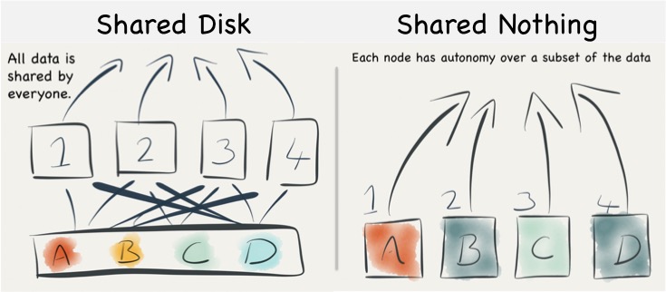
Understanding the Trade-offs for Writing
When persisting data in a shared disk architecture writes can be performed against any node. If node 1 and 2 both attempt to write a tuple then, to ensure consistency with other nodes, the management system must either use a disk based lock table or else communicated their intention to lock the tuple with the other nodes in the cluster. Both methods provide scalability issues. Adding more nodes either increases contention on the lock table or alternatively increases the number of nodes over which lock agreement must be found.
To explain this a little further consider the case described by the diagram below. The clustered shared disk database contains a record with PK = 1 and data = foo. For efficiency both nodes have cached local copies of record 1 in memory. A client then tries to update record 1 so that ‘foo’ becomes ‘bar’. To do this in a consistent manner the DBMS must take a distributed lock on all nodes that may have cached record 1. Such distributed locks become slower and slower as you increase the number of machines in the cluster and as a result can impede the scalability of the writing process.
The other mechanism, locking explicitly on disk, is rarely done in practice as caching is so fundamental to performance.
However shared nothing does not suffer from the same distributed locking problem, assuming that the client is directed to the correct node (that is to say a client writing ‘A’, in the figure above, directs that write at Node 1) , the write can flow straight though to disk with any lock mediation performed in memory. This is because only one machine has ownership of any single piece of data, hence by definition there only ever needs to be one lock.
Thus shared nothing can scale linearly from a write perspective without increasing the overhead of locking data items, because each node has sole responsibility for the data it owns.
However shared nothing will still have to execute a distributed lock for transactional writes that span data on multiple nodes (i.e. a distributed two-phase commit). These are not as large an impedance on scalability as the caching problem above, as they span only the nodes involved in the transaction (as apposed to the caching case which spans all nodes), but they add a scalability limit none the less (and they are also likely to be quite slow when compared to the shared disk case).
So shared nothing is great for systems needing high throughput writes if you can shard your data and stay clear of transactions that span different shards. The trick for this is to find the right partitioning strategy, for instance you might partition data for a online banking system such that all aspects of a user’s account are on the same machine. If the data set can be partitioned in such a way that distributed transactions are avoided then linear scalability, at least for key-based reads and writes, is at your fingertips.
The counter, from the shared disk camp, is that they can use partitioning too. Just because the disk is shared does not mean that data can’t be partitioned logically with different nodes servicing different partitions. There is much truth to this, assuming you can set up your architecture so that write requests are routed to the correct machine, as this tactic will reduce the amount of lock (or block) shipping taking place (and is exactly how you optimise databases like Oracle RAC).
Put another way – a shared disk implementation can be configured in a shared nothing mode. The difference here is just the physical placement of data. Shared disk is always network attached in some way, never local. So whilst remote disks can provide comparatively high throughput and good random IO performance they will do this at often greater monetary cost.
|
Considering the Retrieval of Data
The retrieval of data is a very different story, with different tradeoffs for each of these two approaches. Looking firstly at Shared Disk we find two significant drawbacks:
The first is the potential for resource starvation, most notably disk contention on the SAN/NAS drives. Shared disk means exactly that: all machines share the same disk array, and to some extent the same interconnect. Fortunately disk contention in a large shared disk system can be alleviated by partitioning. Data within the shared disk subsystem is often partitioned by its usage pattern (usually by moving tables onto different sections of the backing disk array). The problem with this approach is that it is manual: the data must be physically partitioned in advance.
The second issue is that caching is less efficient. Each machine in a shared disk system is likely to become involved (and hence have the requirement to cache) the whole dataset. This reduces the efficiency of the cache as cache misses are more likely. This is in stark contrast to the shared nothing approach where each machine only needs to cache the subset of the data that it owns. Thus caching can be far more effective in a shared nothing system.
Shared nothing is not without its flaws though. SN works brilliantly if the query is self sufficient – if each node can complete its ‘portion’ of the processing without needing data from any other node. However there will inevitably arise use cases where data from multiple nodes must be brought together or joined in some way. The implication is often that data, which may not be included in the final result, be shipped from one machine to another. This need to ship data between machines to ‘join’ can have a significant effect of overall query performance.
So the reality is that the number of queries requiring data shipping will depend on both the use case and the partitioning strategy. There are many cases where joins can be eliminated altogether by using Aggregates – for example in commercial search engines. However, for many general business use cases, for example ones with large related fact tables, some data shipping is often inevitable. As a result many shared nothing solutions recommend the use of fast 10GE networks.
Finally we should comment on the concurrency. Many key-value stores use shards and SN to provide very high levels of concurrency. This is achieved by routing user requests, via the sharding key, to the single machine that has the required data. This pattern is very efficient and the result is stores that provide extremely high levels of read and write throughput over a large, concurrent user base. This pattern is used heavily in large web applications via NoSQL.
What we must note is that the scalability of this pattern is only available for key-based access. It does not apply to more general processing in a shared nothing system. Any request that does not explicitly use the primary key must be broadcast to all machines (partitions). This presents a limit to the scalability for questions that do not consider the primary key. As a result many shared nothing systems, which support more general query workloads, show similar levels of concurrency to single node systems (5-10 is not uncommon).
So this is important enough to restate: Shared nothing is only linearly scalable for key-based access. The use of secondary indexes always results in every node being consulted. This limits scalability, certainly in terms of the number of concurrent requests that can be serviced. This is one of the reasons for many distributed key-value stores sticking to the very simple K-V contract.
The retort is that shared nothing reduces the amount of data stored per machine. Thus total data volumes can be higher, or conversely each query will be faster as the average dataset per query is reduced. This is why SN is favoured for Big Data systems like HBase, Map Reduce, Cassandra etc.
|
Complexity at Scale
A possibly less obvious benefit of shared nothing is to do with complexity at scale. Put simply, because of the autonomous nature, each node in a SN system has a relatively simple contract. It’s concerns are encapsulated in its own data partition. This means the software to manage failure can be simpler, behaving with little or no knowledge of it’s wider role in the cluster.
In contrast shared disk systems are fully open to the influence of other nodes. These couplings take the form of locks, with timeouts and relatively complex failure semantics. If we consider a failure in a shared disk system, the node is likely to have locks out on the underlying shared disk structure. These locks implicitly affect the other processing nodes and the system must go through a process of discovering the failed nodes, it’s locks and then releasing them or letting them timeout.
The shared nothing system only has to detect failure and promote the backup node (or similar depending on the failure strategy of the system). In fairness these problems are well understood, but often still misapplied and always bring, IMHO, a little more complexity to bare. Certainly the complexity of these issues seems to grow with the number of nodes and the heterogeneity of the deployment. This means SN often works best for very large installations.
So Which Should You Use?
If you are Google or Amazon then the simple, autonomous SN model will likely be attractive. Key-value based approaches will give you the concurrency you need to serve millions of users. The brute force, divide and conquer approach to data processing will provide the grunt needed to sift through datasets that require hundreds of machines to process.
If you are a business system that is unlikely to need more than two or three servers then the complexities of partitioning a complex domain model efficiently may outweigh the benefits. This is why many business databases such as those provided by Oracle and IBM tend to favour shared disk. Particularly considering a shared disk model can be partitioned to simulate at least some of the benefits of the shared nothing approach but within a shared disk system.
Often the choice is made for you by the implementation, and there may be other features besides the physical architecture that attract you to a certain product. Certainly shared nothing, as an approach, is increasing in popularity. Most of the NoSQL space is shared nothing. However many NoSQLs have blended models that include both sharding and replication as first class primitives. This complicates the picture.
Hadoop also provides a blended model. HDFS is really a type of shared disk but the execution model it uses is shared nothing. Computation is routed to the nodes where data lies, wherever this is possible. Composite models such as this can be attractive as they provide benefits from both approaches: a shared subsystem which spans the various machines in the cluster. A programming model that treats data and processing as shared nothing, with each node assuming an autonomous, local data subset. This provides the benefits of shared nothing’s scaling-through-autonomy but with the power to break from the model where needed. Clever!
So whilst the concept of shared nothing vs shared disk is relatively simple, there are a huge host of other factors that differentiate the data technologies of today. This is just one classifier. But it is a useful one, at least from the perspective of understanding how these different systems work under the hood.
Further Reading
There are a number of good papers on the subject. The infamous Michael Stonebraker was one of the early SN evangelists, back in the early 80’s. His paper The Case For Shared Nothing still makes good reading, even if it does skip some issues.
Also Shared-Disk vs. Shared Nothing by the makers of ScaleDB – a Shared Disk database. This paper makes the case for Shared Disk and enumerates the downsides of Shared Nothing.
The last paper presents the opposite view. How to Build A High Performance Data Warehouse is well written, mapping the pros and cons of each architecture. However don’t be sucked in by the academic URL. The authors are all affiliated with Vertica which is a commercial implementation from the Stonebraker camp, and the paper noticeably favours a Shared Nothing Columnar Architecture model, like the one used by Vertica. Never the less it’s a good read.
Finally there is a good section in Architecture of a Database System.
See also Elements of Scale and Are Databases a Thing of the Past?
Component Software. Where is it going?
Friday, January 14th, 2005
Introduction
In 1943 Thomas Whatson, the then chairman of IBM, infamously announced “I think there is a world market for maybe five computers”. This statement seems quite humorous when quoted in the context of today. Not because it is incorrect, there was undoubtedly sense to his reasoning at the time, but because the context of the statement has been so far lost in the progression that has occurred since.
Whatson observed the trends of his day and attempted to predict the direction of future progression. However, he had no way of predicting details or gauging the rate at which that progression would advance.
Similarly, in this essay we will examine the trends of today, and then reflect on how they can be used to predict the trends of the future. Sudipto Ghosh [Ghosh02] stated that “all future software systems will be developed from components”. We’ll look at this and other opinions on the future of component systems and how they affect the cost efficiency of software projects.
The Future of Components lies in Reuse
Component software today is about two simple concepts, reuse and composition. Re-use is a regular topic of conversation between software engineers. We often discuss the merits of abstracting a class so that it can be packaged or wrapped, allowing customers to utilise its functionality directly. However in other branches of engineering you would find little discussion on this or related topics. This is not because reuse is specific to Software Engineering. On the contrary, engineers are expert in selecting and reusing appropriate components in their work. It is the fact that reuse is so commonplace in engineering that makes it, for them, an uncontroversial topic.
Engineers are taught, from their very first lectures, the art of balancing the trade-offs of different components when selecting the most appropriate one for the situation.
Software engineers on the other hand are generally not so good at reuse. Software engineering is still in a “craftsmanship” phase that leads more naturally to rewrite rather than reuse.
The problem is that software is a soft and malleable product that can be moulded into whatever exact shape suits. The question then arises as to whether this perceived advantage of the “softness of software” is really a liability?
One argument, put forward by Ruben Prieto-Diaz [Prieto96], is that the progression of software engineering as a discipline can only really come through the toughening of standards and conventions to impose structure on the pliability of the discipline. He believes that only when software becomes less malleable will reuse, in the forms seen in other engineering disciplines, become practical.
Ruben’s findings still bear much relevance to the evolution and progression of component software today. This issue of the softness of software is still pertinent and, as we shall see, many future developments are geared to restricting the directions in which software can be stretched.
Ruben’s foresight was not only limited to the need for increased structure and standards. He also observed that it is complexity that promotes reuse. His principal states that the more complex a software component the greater the motivation for reusing it (as apposed to rewriting from scratch). This concept points to the inevitability of components within software engineering thus paving the way for the future we see today.
The Future of Components lies in Composition
A different and slightly later view to Ruben’s was put forward by Bennet [Benn00] who considered not only reuse but also the aspect of composition, which is a fundamental contributory element of component software. He notes that over the last half-century software processes have been dominated by managing the complexities of the development and deployment of increasingly sophisticated systems.
Bennett’s view is that there needs to be a shift in the focus of software towards users rather than developers. He states that software development needs to be more demand-centric so as to allow it to be delivered as a service within the framework of an open marketplace. The concept being introduced is known as a Service Based Approach to Software and the analogy he uses is one of selling cars.
Historically cars were sold from pre-manufactured stock but increasingly nowadays consumers configure their desired car from a series of options and only then is the final product assembled. The comparable process in software is to allow users to create, compose and assemble a service, dynamically bringing together a number of different suppliers to meet the consumer’s needs.
The issues imposed by such a proposal lie in the complexities involved in the late binding of software components. Bennet suggests his research will be able to perform binding delayed until the point of execution. This allows customers to select the various components of their systems from a potential variety of vendors and from these components build the customised system of their choice, a concept known as adaptable composition.
These ideas of adaptable composition are extended even further into the future by Howard Shrobe [Shrobe99] in his paper of The Future of Software Technology [Shrobe99]. Shrobe presents an interesting view of the future as one composed of self-adaptive systems that are sensitive to the purposes and goals of the components from which they are composed. Such systems would contain multiple components with similar but slightly disparate roles and the runtime would be able to dynamically determine the most appropriate component for a certain task.
In particular he comments on the long-standing wider research aims to develop tools and methodologies with make impenetrable and properly correct systems. Shobe doubts the usefulness of such methods in future systems. He believes that many of the problems that require such measures arise from the harshness and unpredictability of the environment rather than the mental limitations of programmers.
Instead, he suggests that a range of techniques and tools will emerge that facilitate the construction of inherently self-adaptive systems and goes on to predict some of their features. These will include multiple components being available for any single task. The most appropriate one being selected dynamically by the runtime environment. This is what he calls a Dynamic Domain Architecture. Such architectures are more introspective and reflective that conventional systems. The key elements being:
- Monitors that will check validation conditions are true at various points.
- Diagnosis and isolation services that will determine the cause of exceptional conditions.
- Services will be available that select alternative components to use in the event of failure.
Such systems will need to be, in some ways, self-aware and goal directed. Shobe also foresees the interactions between developers and the system taking the form of a dialogue rather than coding. The developer would offer advice to the system at certain critical points to aid its’ judgement in how to deal with different situations.
Are these futures realistic?
The views of both Bennet and Shrobe are fairly far reaching. Shrobe’s in particular represents a quite extreme vision. However all the ideas so far are grounded in the fundamentals of how component software (and software in general) is developed today.
To see how such views can be considered plausible it is useful to consider the motivations for Component Software expressed by other prominent authors. Clemens Szyperski, one of the fathers of Component Software, explores the motivations for current and future trends in component software in his paper Component Software: What, Where and How? [Szyp02]. Here he divides the motivations for using software components into the four tiers summarised below:
Tier 1: Build Time Composition
Component applications that reside in this tier use prefabricated components in amongst custom development. This drives balance between the competitive advantages of purpose-built software and the economic advantage of standard purchased components. Most importantly components are consumed at development time and released as part of a single custom implementation.
Tier 2: Software Product Lines
Scaling above Tier 1 involves the reuse of partial designs and implementation fragments across multiple products. This is the domain of Software Product Lines [Web1], [Bosch00]. In this tier components are developed for reuse across multiple products. This is similar in some ways to conventional manufacture. An automotive manufacturer may create a variety of unique variations of a single car model. These would be constructed through the use of standard components and production systems that specialise in their configuration and assembly into the various products. A similar concept can be applied to component development and assembly with developers taking roles either as component assemblers or product integrators.
Tier 3: Deployment Composition
In this tier components are integrated as part of the product’s deployment (not at build time). An example of deployment composition is the web browser, which is deployed then subsequently updated with downloaded components that enable specialist functionality on certain web pages. Sun’s J2EE also supports partial composition at deployment time through the use of a deployment descriptor and hence also falls into this category.
Tier 4: Dynamic Upgrade and Extension
In this final tier there are varying degrees of redeployment and automatic installation that facilitate a product that can grow and evolve over its lifetime. This final tier is the realm of current and future research.
What is notable about Szyperski’s tiers is that they are all motivated by financial drivers. Tier1 arises from the competitive advantage gained through reusing prefabricated components over developing them in house. Tier2 results from the forces of an economy scope[1] to extend reuse beyond singular product boundaries and into orchestrated reuse programmes.
In the third and fourth tiers Szyperski switches focus from just reuse to aspects of composition and dynamic upgrade. However the economic motivators here are subtler.
In the third tier they focus on the need for standardisation in a similar vein to that introduced earlier by Prieto-Diaz. Deployment composition generally relies on a framework within which the components operate. This introduces a much-needed discipline to the process as well as offering the opportunity to develop components, which leverage off the framework itself.
The fourth tier supports dynamic upgradeable and extensible structures and represents Syperski’s view on the future of component software. Research into applications in this tier provides an extremely challenging set of problems for researchers, such as validation of correctness, robustness and efficiency.
With this fourth tier architecture Szyperski is pointing towards a future of dynamic composition but also notes that it is one that it will likely be hindered by the problems of compositional correctness. Validating dynamically composed components in a realistic deployment environment is an extremely complex problem simply as a result of the implementation environment not being known at the time of development.
This is an issue of quality assurance. Firstly there is no reliable means to exhaustively test integrations at the component suppliers end. Secondly there are little in the way of component development standards, certifications or best practices that might help increase consumer confidence in software components by guaranteeing the reliability of vended components.
David Garlan [Gar95] illustrated similar issues a decade ago in the domain of static component assembly. Garlan noted problems with low-level interoperability and architectural mismatch resulting from incompatibilities between the components he studied. Issues such as “which components hold responsibility for execution” or “what supporting services are required” are examples of problems arising from discrepancies in the assumptions made by component vendors.
Garlan listed four sets of improvements which future developments must incorporate to overcome the problems of interoperability and architectural mismatch:
- Make architectural assumptions explicit.
- Construct large pieces of software using orthogonal sub-components.
- Provide techniques for bridging mismatches
- Develop sources of architectural design guidance.
Whilst these issues were observed when considering static composition (i.e. within Szyperski’s first Tier) the same issues are applicable to higher tiers too. Approaches to remedying these issues have been suggested on many levels. One approach is to provide certification of components so that consumers have some guarantee of the quality, reliability and the assumptions made in their construction. Voas introduced a method to determine whether a software component can negatively affect an utilising system [Voas97].
The same concept has been taken further at the Software Engineering Institute (SEI) at Caregie Mellon with a certification method known as Predictable Assembly from Certifiable Components or PACC [Web2]. Instead of simple black box tests PACC allows component technology to be extended to achieve predictable assembly using certified components. The components are assessed though a validation framework that measurers statistical variations in various component parameters (such as connectivity and execution ranges). This in turn allows companies greater confidence in the reliability of the components they assemble.
Szyerski also alludes to a similar conclusion:
“Specifications need to be grounded in framework of common understanding. At the root is a common ontology ensuring agreed upon terminology and domain concepts.” [Szyper02].
He suggests the solution of a specification language, AsmL, which shares some similarities with PACC. AsmL, which is based on the concept of Abstract State Machines [Gure00], is a means for capturing operational semantics at a level of abstraction that fits in with the process being modelled. Put another way it allows the formalisation of the operations and interactions of the components that it describes in a type of an overly rich interface description. This in turn allows processes to be specified and validated with automated test case generators thus providing verification and correctness by construction.
AsmL has been applied on top of Microsoft’s .NET CLR by Mike Barnet et al. [Barn03] with some successes made in specifying and verifying correctness of composed component systems. In Barnet’s implementation the framework is able to provide notification that components do not meet the required specification (along similar lines to that suggested by Shrobe) but is as yet unable to provide automated support or actually pinpoint the reason for the failure.
Keshava Reddy Kottapally [Web3] presents a near and far future view of component software as being influenced by the development of Architectural Description Languages (ADL’s). These ADL’s focus on the high level structure of the overall application rather then implementation details and again arise from similar concepts to those suggested by Szyperski. Physically they provide specification of a system in terms of components and their interconnections i.e. they describe what a component needs rather than what it requires.
Kottapally’s near future view revolves around adaptation of the currently prominent component architectures (.NET, J2EE, CORBA) to incorporate ADL’s. He gives the example that ADL files would be built with Builder tools designed specifically for ADL specification. Then interfaces such as CORBA IDL could be generated automatically once the ADL file is in place. The purpose being to facilitate connection orientated implementations where the connections can handle different data representations. This would be enabled via bridges between interoperability standards (e.g. a CORBA EJB Bridge).
He also suggests a unified move to the new challenges proposed by COTS based development. COTS-Based Systems focus on improving the technologies and practices used for assembling prefabricated components into large software systems [COTS04], [Voas98]. This approach attempts to realign the focus of software engineering from the traditional linear process of system specification and construction to one that considers the system contexts such as requirements, cost, schedule, operating and support environments simultaneously.
Kottapally continues to present a more far-reaching view on the future of CBSD. In particular he highlights several developments he feels are likely to become important:
- The removal of static interfaces to be replaced by architectural frameworks that deal with name resolution via connectors.
- Resolution of versioning issues.
- General take up of COTS
- Traditional SE transforms to CBSD.
- Software agents will represent human beings acquiring intelligence and travelling in the global network using component frameworks and distributed object technologies.
Components are Better as Families
So far we have seen evidence that the future of component software is likely to be grounded in the issues that facilitate both the static and dynamic composition within software products. We have also seen that some efforts have already been made to increase the rigidity of the environments in which these products operate thus allowing compositions to become more reliable. However there is another set of views on how we achieve these truly composable systems that originate from a slightly different tack.
Greenfield et al [SoftFact] foresee a more systematic approach to reuse arising from the integration of several critical innovations to produce a process akin to the industrialisations observed in other industries. This goes somewhat beyond the realm of Component Software and considers issues such as the development of domain specific languages and tools to reduce the amount of handwritten code. However they do express several interesting opinions on the application of component software in their vision of the future.
Greenfield et al make two statements in particular that encapsulate what they feel to be the most critical developments in component software:
- “Building families of similar but distinct software products to enable a more systematic approach to reuse”.
- “Assembling self-describing service components using new encapsulation, packaging, and orchestration technologies”.
The first point refers to the systematic approaches, such as Software Product lines that were introduced earlier. Studies have shown [Clem01] that the applications of Software Product Line principals allow levels of reuse in excess of two thirds of the total utilised source (a level that would be difficult to achieve through regular component assembly methods).
Greenfield puts forward the view that the environment of software development will be fundamentally changed by the introduction of such high levels of reuse. This in turn will induce the arrival of software supply chains.
Supply chains are a chain of states with raw materials at one end and a finished product at the other. The intermediate steps involve participants combining products from upstream suppliers, adding value then passing them on down the chain. Greenfield claims that the introduction of supply chains will act as a force to standardise. Something observed as a necessity by most authors on the subject of software component evolution.
Greenfield’s second point, listed above, refers to the concept of Self-Description. Self-Description allows components to describe the assumptions, dependencies and behaviour that are intrinsic to their execution, thus providing operational as well as contractual data. This level of meta-data will allow a developer or even a system itself to reason about the interactions between components.
This idea is extended further via the extension of modelling languages, such as UML, to a level that allows them to describe development rather than just providing documentation of the development process. In such a vision the modelling language forms an integral part of the deployment.
There are similarities here to the concept of AsmL put forward by Szyerski earlier. In addition Greenfield, like Szyerski, also emphasises the need for executing platforms to proceed to higher levels of abstraction:
“Together these lead to the prospect of an architecturally-driven approach to model-driven development of product families”. ([SoftFact] p452)
It is also interesting to note that the concept of self-description follows on logically from the points Garlan made earlier regarding architectural assumptions being explicit and the bridging of architectural mismatches.
So what of the future?
Components are primarily designed for composition. One of the main attractions of any component-based solution is the ability to compose and recompose the solution using products from potentially different vendors. We have seen examples of issues with static composition raised over a decade ago [Gar95] and the same issues are pointed out time and time again ([Szyp02], [GSCK04], [Voas97], [Web3], [SzypCS]). We have seen solutions suggested including self-description and ADL’s. However one of the main aims is to produce agile software constructions and this includes the ability to compose systems dynamically, even at runtime.
Whether these visions actually come into being is difficult to say. It is certainly true that the interactions in these structures are increasingly complex and that already there are observable tradeoffs to be made by developers with respect to performance versus compositional variance (as highlighted currently with frameworks such as Suns J2EE). In the next section we will consider the financial implications of component technologies and attempt to determine whether they actually provide practical cost benefits for consumers both now and in the future.
Are Component Technologies Cost Effective?
Szyperski’s four motivational tiers that were introduced earlier coupled with the fact that each increasing tier requires more refined competencies leads to the concept of a Component Maturity Model [Szyp02]. The levels are distinguished as:
1. Maintainability: Modular Solutions.
2. Internal Reuse: product lines.
3a. Closed Composition: make and buy from a closed pool of organisations
3b. Open Composition: make and buy from open markets
4. Dynamic Upgrade
5. Open and Dynamic
To consider the cost effectiveness of component software it is convenient to consider the financial drivers within each of these levels.
Level 1. Maintainability: Modular Solutions.
At this level components are produced in house and reused within a project. The aim from an economic standpoint is to reduce costs by promoting reuse. From a development position the “rule of thumb” is that a component becomes cost effective once it has been reused three times [SzypCS]. This property emerges from the trade off between the cost of redeveloping a component when it is needed against the increased initial cost of an encapsulated and reusable solution. This relationship is shown in fig 1.
Make architectural assumptions explicit
Economic returns are generally increased further when maintenance costs are also considered due to the lower maintenance burden of a single (if slightly larger) source object.
Level 2. Internal Reuse: Product Lines
Internal reuse in the form of product lines, as introduced earlier, involves reusing internally developed components across a range of similar products within a product line. The economic impact is multifaceted. Product lines increase efficiency as they dramatically increase the level of component reuse that can be sustained in a development cycle. However these rewards reaped from the cross asset utilisation of shared components must be offset against the increased managerial and logistical stresses imposed by such an interdependent undertaking.
Level 3a/b. Closed Composition:
Make and buy from a closed/open market of organisations
We have seen that there is significant evidence to suggest economic advantage from the use of modular development. The economic advantages of reuse in an OO sense are compulsive and this fact alone was a major factor in the success of the object-orientated revolution of the end of the last century. However it is when this concept is extended to reuse across company boundaries that the economic benefits become really interesting.
Component reuse offers the potential for dramatic savings in development costs if executed successfully. Never before has the concept of non-linear productivity been on offer to software organisations. Quoting Szyperski [SzypCS]:
“As long as solutions to problems are created from scratch [i.e. regular development], growth can be at most linear. As components act as multipliers in a market, growth can become exponential. In other words, a product that utilises components benefits from the combined productivity and innovation of all component vendors”.
The use of prefabricated components offers the potential to compose hugely complex software constructions at a fraction of their development cost simply by purchasing the constituent parts and assembling them to form the desired product. It is this promise of instant competitive advantage, which makes the use of components so compulsive, and it is this that makes them truly cost effective.
In fact the dynamics of a software market fundamentally changes when components are introduced. When a certain domain becomes large enough to support a component market of sufficient size, quality and liquidity the creation of that market becomes inevitable. The adoption of components by software developers then becomes a necessity. Standard solutions are forced to utilise these components in order to keep up with competitors. At this point competitive advantage can then only be achieved by adding additional functionality to that offered by the composition of available components within the software market.
The important balance to consider is one between the flexibility, nimbleness and competitive edge provided by regular programming and the cost efficiencies provided by reusing prefabricated components. This relationship is shown in fig 2.

This concept of development by assembly was in fact one of the important changes promulgated by the industrial resolution. The advent of assembly lines marked the transition from craftsmanship to industrialisation. The analogy is useful when considering software development to also be in a period of craftsmanship and hence inferring that taking the same steps will bring industrialisation to the software industry. However a number of subtle differences have manifested themselves that have resulted in little of the predicted revolution in component utilisation actually taking place.
This slowness in take up can be attributed to a number of factors:
- Lack of liquidity in component markets: Many markets lack liquidity or companies fail to address the difficult marketing issues provided by an immature market such as component software.
- Integration issues such as platform specific protocols.
- Lack of transparency in component solutions and weak packaging. Black box solutions often hide true implementation details and documentation can be weak.
- Reliability issues. Black/Glass box solutions can prove problematic for customers as minor inaccuracies in product specification can prove challenging or impossible to fix.
- Raising issues back to the vendor is rarely a practical solution.
- The “not invented here” syndrome. Suspicion of vendor components leads to the dominance of in-house construction. In addition components that are used are often only applied in opportunistic manners rather than as an integrated part of the design.
Points 3, 4 and 5 represent the major differences between closed pool and open market acquisition. The closed pool allows companies greater confidence in the component manufacture through the building of a mutually beneficial relationship between client and vendor. However the reduction in breadth of components available restricts the opportunity for full leverage from the component market at large.
Level 4+5. Open and Dynamic Upgrade:
The efficiency of dynamic upgrade is easy to judge as what technology is currently implelmentable is of too unreliable a form to be efficient. However future applications of dynamic upgrade are likely to appear in performance orientated environments that can reap large benefits from the extra flexibility offered. Applications such as mobile phone routing are potential candidates where the opportunity to dynamically switch in and out encapsulated components in a hot system is highly valued due to the avoidance of down time.
Conclusions
So is component software cost efficient? The answer to this question, as with many, lies in the context in which it is asked. The efficiency of component software varies according the maturity level at which it is applied. At lower levels economic benefits arise from reuse as part of the development process. This has a significant if not exceptional effect on efficiency.
As utilisation moves to a level that consumes vendor components, the potential for economic advantage increases dramatically. Companies at this maturity level can achieve exponential product growth. Hence, in answer to the question posed, component software provides the possibility for substantial increases in cost efficiency. But this potential is, as yet, unrealised in most software markets. This lack of take up of component software can be traced to two specific and interdependent aspects:
On one side is the ideology of software engineering itself. Software engineers are brought up to develop software rather than assemble components. It is only natural that they should favour the comforts of an environment they are familiar with over the foreboding challenges imposed by the world of assembly.
On the other hand there are significant problems with the components of today resulting from issues of their implementation in general, which makes them hard to use.
As we look to the future, and component markets mature, it is likely that the issues of integration highlighted earlier in the paper will be resolved. This in turn should induce closer relationships between customers and suppliers, strengthening the process as well as increasing confidence in assembly as a practical and reliable methodology for industrial application construction.
But the future is a hard thing to predict. The world contains a substantially larger number of computers than Whatson originally predicted. This does not mean Whatson was wrong though. It simply means it has not, yet, been proved right. It is entirely possible that we may end up with a world containing only a handful of computers, depending of course, on your definition of a computer. The reality though is that, when it comes to the future, the only truly accurate option is to simply wait and see.
References
[Barn03] Barnet et al: Serious Specification for Composing Components 6th ICSE Workshop on Component-Based Software Engineering
[Benn00] Service-based software: the future for flexible software, K. Bennett, P. Layzell, D. Budgen, P. Brereton, L. Macaulay, M. Munro: Seventh Asia-Pacific Software Engineering Conference (APSEC’00)
[Bosch00] j. Bosch: Design and use of software architectures: Adopting and evolving a product line approach. Addison Wisley 2000
[Clem01] Software Product Lines: Practices and Patterns: Clements and Northrop
[COTS04] http://www.sei.cmu.edu/cbs/overview.html
[Gar95] David Garlan: Architectural Mismatch of Why it’s hard to build a system out of existing parts.
[Ghosh02] “Improving Current Component Development Techniques for Successful Component-Based Software Development,” S. Ghosh. 7th International Conference on Software Reuse Workshop on Component-based Software Development Processes, Austin, April 16, 2002.
[GSCK04] Software Factories: Greenfield, Short, Cook and Kent. Wiley 2004
[Gure00] Y. Gurevich: Sequential Abstract State Machines Capture Sequential Algorithms: ACM Transactions on Computational Logic.
[Pour98] Gilda Pour: Moving Toward Component-Based Software Development Approach 1998 Technology of Object-Oriented Languages and Systems
[Prieto96] Ruben Prieto-Diaz: Reuse as a New Paradigm for Software Development. Proceeding of the International Workshop on Systematic Reuse. Liverpool 1996.
[Shrobe99] Howard Shrobe, MIT AI Laboratory, Software Technology of the Future 1999 IEEE Symposium on Security and Privacy
[Szyp02] Clemens Szyperski: Component Technology – What, Where and How?
[SzypCS] Clemens Szyperski: Component Software – Beyond Object-Orientated Programming. Second Edition Addison-Wesley
[Voas97] Jeffrey Voas: An approach to certifying off-the-shelf software components 1997
[Voas98] Jeffery Voas: The Challenges of Using COTS Software in Component-Based Development (Computer Magasine)
[Web1] http://www.softwareproductlines.com/
[Web2] http://www.sei.cmu.edu/pacc
[Web3] Keshava Reddy Kottapally: ComponentReport1: http://www.cs.nmsu.edu/~kkottapa/cs579/ComponentReport1.html
[1] Software is subject to the forces of an economy of scope rather than and economy of scale. Economies of scale arise when copies of a prototype can be mass-produced at reduced cost via the same production assets. Such forces do not apply to software development where the cost of producing copies is negligible. Economies of scope arise when production assets are reused but to produce similar but disparate products.
Do Metrics Have a Place in Software Engineering Today?
Sunday, March 14th, 2004
Introduction
The famous British physicist Lord Kelvin (1824-1904) once commented:
“When you can measure what you are speaking about, and express it in numbers, you know something about it; but when you cannot measure it, when you cannot express it in numbers, your knowledge is of a meagre and unsatisfactory kind. It may be the beginning of knowledge, but you have scarcely, in your thoughts, advanced to the stage of science.”
This statement, when applied to software engineering, reflects harshly upon the software engineer that believes themselves to really be a computer scientist. The fundamentals of any science lie in its ability to prove or refute theory through observation. Software engineering is no exception to this yet, to date, we have failed to provide satisfactory empirical evaluations of many of the theories we hold as truths.
I take the view that comprehensibility should be the main driver behind software design, other than satisfying business and functional requirements, and that the route to this goal lies in minimisation of code complexity. Software comprehension is an activity performed early in the software development lifecycle and throughout the lifetime of the product and hence it should be monitored and improved during all phases. In this paper I will reflect specifically on methods through which software metrics can aid the software development lifecycle through their ability to measure, and allow us to reason about, software complexity.
Kelvin says that if you cannot measure something then your knowledge is of an unsatisfactory kind. What he is most likely alluding to in this statement is that any understanding that is based on theory but lacks qualitative support is inherently subjective. This is a problem prevalent within our field. Software Engineering contains a plethora of self-appointed experts promoting their own, often unsubstantiated, views. Any scientific discipline requires an infrastructure that can prove or refute such claims in an objective manner. Metrics lie at the essence of observation within computer science and are therefore pivotal in this aim.
In the conclusion to this paper I reflect on the proposition that metrics are more than just a way of optimising system construction, they provide the means for measuring, reasoning about and validating a whole science.
Measuring Software
Software measurement since its conception in the late 1960’s has striven to provide measures on which engineers may develop the subject of Software Engineering. One of the earliest papers on software metrics was published by Akiyama in 1971 [8].
Akiyama attempted to use metrics for software quality prediction through a crude regression based model that measured module defect density (number of defects per thousand lines of code). In doing this he was one of the first to attempt the extraction of an objective measure of software quality through the analysis of observables of the system. To date defect counts form one of the fundamental measurements of a software system (although a general distinction between pre and post release defects is usually made).
In the following years there was an explosion of interest in software metrics as a means for measuring software from a scientific standpoint. Developments such as Function Point measures pioneered in 1979 by Albrecht [17] are a good example. The new field of software complexity also gained a lot of interest, largely pioneered by Halstead and McCabe.
Halstead proposed a series of metrics based on studies of human performance during programming tasks [11]. They represent composite, statistical measures of software complexity using basic features such as number of operands and operators. Halstead performed experiments on programmers that measured their comprehension of various code modules. He validated his metrics based on their performance.
McCabe presented a measure of the number of linearly independent circuits through the program [10]. This measure aims specifically to gauge the complexity within the software resulting from the number of distinct routes through a program.
The advent of Object Orientation in the 1990’s saw a resurgence of interest as researches attempted to measure and understand the issues of this new programming paradigm. This was most notably pioneered by Chidamber and Kemerer [2] who wrapped the basic principals of Object Orientated software construction in a suite of metrics that aim to measure the different dimensions of software.
This metrics suite was investigated further by Basili and Briand [25] who provided empirical data that supported their applicability as measures of software quality. In particular they note that the metrics proposed [2] are largely complementary (see later section on metrics suites).
These metrics not only facilitate the measurement of Object Orientated systems but also lead to the development of a conceptual understanding of how these systems act. This is particularly notable with metrics like Cohesion and Coupling which a wider audience now considers as basic design concepts rather than just software metrics. However questions have been raised over their correctness from a measurement theory perspective [26,27,30] and as a result optimizations have been suggested [31].
A second complimentary set of OO metrics was proposed by Abreu in 1995 [32]. This suite, denoted the Mood Metrics Set, encompasses similar concepts to Chidamber and Kemerer but from a slightly different, more system wide, viewpoint on the system.
To date there are over 200+ documented software metrics designed to measure and assess different aspects of a software system. Fenton [12] states that the rationale of almost all individual metrics for measuring software has been motivated by one of the two activities: –
1. The desire to assess or predict the effort/cost of development processes.
2. The desire to assess or predict quality of software products.
When considering the development of proper systems, systems that are fit for purpose, the quality aspects in Fenton’s second criteria, in my opinion, outweigh those of cost or effort prediction. Software quality is a multivariate quantity and its assessment cannot be made by any single metric [12]. However one concept that undoubtedly contributes to software quality is the notion of System Complexity. Code complexity and its ensuing impact on comprehensibility are paramount to software development due to its iterative nature. The software development process is cyclical with code often being revisited frequently for maintenance and extension. There is therefore a clear relationship between the costs of these cycles and the complexity and comprehensibility of the code.
There are a number of attributes that drive the complexity of a system. In Software Development these include system design, functional content and clarity. To determine whether metrics can help us improve the systems that we build we must look more closely at Software Complexity and what metrics can or cannot tell us about its underlying nature.
Software complexity
The term ‘Complexity’ is used frequently within software engineering but often when alluding to quite disparate concepts. Software complexity is defined in IEEE Standard 729-1983 as: –
“The degree of complication of a system or system component, determined by such factors as the number and intricacy of interfaces, the number and intricacy of conditional branches, the degree of nesting, the types of data structures, and other system characteristics.”
This definition has widely been recognized as a good start but lacking in a few respects. In particular it takes no account of the psychological factors associated with the comprehension of physical constructs.
Most software engineers have a feeling for what makes software complex. This tends to arise from conglomerate of different concepts such as coupling, cohesion, comprehensibility and personal preferences. Dr. Kevin Englehart [19] divides the subject into three sections: –
– Logical Complexity e.g. McCabes Complexity Metric
– Structural Complexity e.g. Coupling, Cohesion etc..
– Psychological/Cognitive/Contextual Complexity e.g. comments, complexity of control flow.
Examples of logical and structural metrics were discussed in the previous section. Psychological/Cognitive metrics have been more of a recent phenomenon driven by the recognition that many problems in software development and maintenance stem from issues of software comprehension. They tend to take the form of analysis techniques that facilitate improvement of comprehension rather than actual physical measures.
The Kinds of Lines of Code metric proposed in [28] attempts a measure cognitive complexity through the categorization of code comprehension at its lowest level. Analysis with this metrics gives a measure of the relative difficulty associated with comprehending a code module. This idea was developed further by Rilling et al [33] with a metric called Identifier Density. This metric was then combined with static and dynamic program slicing to provide a complementary method for code inspection.
Consideration of the more objective, logical and structural aspects of complexity is still a hugely challenging task, due to the number of factors that contribute to the overall complexity of a software system. In this paper I consider complexity to comprise all three of the aspects listed above but note that there is a base level associated with any application at any point in time. The complexity level can be optimized to refractor sections that are redundant or accidentally complex but a certain level of functional content will always have a corresponding base level of complexity.
Within research there has been, for some, a desire to identify a single metric that encapsulates software complexity. Such a consolidated view would indeed be hugely beneficial, but many researchers feel that such a solution is unlikely to be forthcoming due to the overwhelming number of, as yet undefined, variables involved. There are existing metrics that measure certain dimensions of software complexity but they do so often only under limited conditions and there are almost always exceptions to each. The complex relationships between the dimensions, and the lack of conceptual understanding of them, adds additional complication. George Statks illustrates this point well when he likens Software Complexity to the study of the weather.
“Everyone knows that today’s weather is better or worse than yesterdays. However, if an observer were pressed to quantify the weather the questioner would receive a list of atmospheric observations such as temperature, wind speed, cloud cover, precipitation: in short metrics. It is anyone’s guess as to how best to build a single index of weather from these metrics.”
So the question then follows: If we want to measure and analyze complexity but cannot find direct methods of doing so, what alternative approaches are likely to be most fruitful for fulfilling this objective?
To answer this question we must fist delve deeper into the different means by which complex systems can be analyzed.
Approaches to Understanding Complex Systems
There are a variety of methods for gathering understanding about complex systems that are employed in different scientific fields. In the physical sciences systems are usually analyzed by breaking them into their elemental constituent parts. This powerful approach, known as Reductionism, attempts to understand each level in terms on the next lower level in a deterministic manner.
However such approaches become difficult as the dimensionality of the problem increases. Increased dimensionality promotes dynamics that are dominated by non-linear interactions that can make overall behaviour appear random [20].
Management science and economics are familiar with problems of a complex, dynamic, non-linear and adaptive nature. Analysis in these fields tends to take an alternative approach in which rule sets are derived that describes particular behavioural aspects of the system under analysis. This method, known as Generalization, involves modelling trends from an observational perspective rather than a Reductional one.
Which approach should be taken, Reductionism or Generalization, is decided by whether the problem under consideration is deterministic. Determinism implies that the output is uniquely determined by the input. Thus a prerequisite for a deterministic approach is that all inputs can be quantified directly and that all outputs can be objectively measured.
The main problem in measuring the complexity of software through deterministic approaches comes from difficulty in quantifying inputs due to the sheer dimensionality of the system under analysis.
As a final complication, software construction is a product of human endeavour and as such contains sociological dependencies that prevent truly objective measurement.
Using metrics to create multivariate models
To measure the width of this page you might use a tape measure. The tape measure might read 0.2m and this would give you an objective statement which you could use to determine whether it might fit it in a certain envelope. In addition the measurement gives you a conceptual understanding of the page size.
Determining whether it is going to rain is a little trickier. Barometric pressure will give you an indicator with which you make an educated guess but it will not provide a precise measure. Moreover it is difficult to link the concept of pressure with it raining. This is because the relationship between the two is not defining.
What is really happening of course is that pressure is one of the many variables that together contribute to rainfall. Thus any model that predicts weather will be flawed if other variables, such as temperature, wind speed or ground topologies are ignored.
The analysis of Software Complexity is comparable to this pressure analogy in that there is disparity between the attributes that we can currently measure, the concepts that are involved and the questions we wish answered.
Multivariate models attempt to combine as many metrics as are available in a way that maximizes the dimension coverage within the model. They also can examine the dependencies between variables. Complex systems are characterized by the complex interactions between these variables. A good example is the duel pendulum which, although being only comprised of two single pendulums, quickly falls into a chaotic pattern of motion. Various multivariate techniques are documented that tackle such interdependent relationships within software measurement. They can be broadly split into two categories:
1. The first approach notes that it is the dependencies between metrics that form the basis for complexity. Thus examination of these relationships provides analysis that is deeper than that created with singular metrics as it describes the relationship between metrics. Halstead’s theory of software science [2] is probably the best-known and most thoroughly studied example of this.
2. The second set is more pragmatic about the issue. They accept that there is a limit to what we can measure in terms of physical metrics and they suggest methods by which those metrics available can be combined in a way that maximizes benefit. Fenton’s Bayesian Nets [4] are a good example of this although their motivation is more heavily focused on the prediction of software cost than the evaluation of its quality.
Metrics suites
One of the popular methods for dealing with the multi dimensionality of complexity is by associating different metrics within a metrics suite. Methods such those discussed in [13], [14] follow this approach. The concept is to select metrics that are complementary and together give a more accurate overview of the systems complexity that each individual metric would alone.
Regression Based and stochastic models
The idea of combining metrics can be extended further with regression-based models. These models use statistical techniques such as factor analysis over a set of metrics to identify a small number of unobservable facets that give rise to complexity.
Such models have had some success. In 1992 Borcklehurst and Littlewood [21] demonstrated that a stochastic reliability growth model could produce accurate predictions of the reliability of a software system providing that a reasonable amount of failure data can be collected.
Models like that produced by Stark and Lacovara [15] use factor analysis with standard metrics as observables. The drawback of these methods is that the resulting models can be difficult to interpret due to their “black box” analysis methodologies. Put another way; the methods by which they analyze cannot be attributed to a causal relationship and hence their interpretation is more difficult.
Halstead [23] presented a statistical approach that looks at total number of operators and operands. The foundation of this measure is rooted in information theory – Zipf’s laws of natural languages, and Shannon’s information theory. Good agreement has been found between analytic predictions using Halstead’s model and experimental results. However, it ignores the issues of variable names, comments, choice of algorithms or data structures. It also ignores the general issues of portability, flexibility and efficiency.
Causal Models
Fenton [12] suggests an alternative that a uses a causal structure of software development which makes the results much easier to interpret. His proposal utilizes Bayesian Belief Networks. These allow those metrics that are available within a project to be combined in a probabilistic network that maps the causal relationships within the system.
These Bayesian Belief Nets also have the added benefit that they include estimates of the uncertainly of each measurement. Any analytical technique that attempts to provide approximate analysis must also provide information on the accuracy of the results and this is a strong benefit with this technique.
Successes and Failures in Software Measurement
In spite of the advances in measurement presented by the various methods discussed above there are still problems evident in the field. The disparity between research into new measurement methods and their uptake in industrial applications highlight these problems.
There are 30+ years of research into software metrics and far in excess of 200 different software metrics available yet these have barely penetrated the mainstream software industry. What has been taken up also tends to be based on the many of the older metrics such as Lines of code, Cyclometric Complexity and Function points which where all developed in or before the 1970’s.
The problem is that prospective users tend to prefer the simpler, more intuitive metrics such as lines of code as they involve none of the rigmarole of the more esoteric measures [12]. Many metrics and consolidation processes lack strong empirical backing or theoretical frameworks. This leaves users with few compelling motivations for adopting them. As a result these new metrics rarely appear any more reliable than their predecessors and are often difficult to digest. These factors have contributed to their lack of popularity.
However metrics implemented in industry are often motivated by different drivers to those of academia. Their utilization is often motivated by a desire to increase certification levels (such as CMM [22]). They are sometimes seen as something used as a last resort for projects that are failing to hit quality or cost targets. This is quite different from the academic aim of producing software of better quality or rendering more effective management.
So can metrics help us build better systems?
Time and cost being equal and business drivers aside, the goal of any designer is to make their system easy to understand, alter and extend. By maximizing comprehensibility and ease of extension the designer ensures that the major burden in any software project, the maintenance and extension phases are reduced as much as possible.
In a perfect word this would be easy to achieve. You would simply take your “complexity ruler” and measure the complexity of your system. If it was too complex you might spend some time improving the design.
However, as I have shown, there is no easily achievable “complexity ruler”. As we have seen software complexity extends into far more dimensions that we can currently model with theory, not to mention accurately measure.
But nonetheless, the metrics we have discussed give useful indicators for software complexity and as such are a valuable tool within the development and refactoring process. Like the barometer example they give an indicator of the state of the system.
Their shortcomings arise from the fact that they must be used retrospectively when determining software quality. This fact arises as metrics can only provide information after the code has been physically put in place. This is of use if you are a manager in a large team trying to gauge the quality of the software coming from the many developers you may oversee. It is less useful when you are trying to prevent the onset of excessive or accidental complexity when designing a system from scratch. Reducing complexity through refactoring retrospectively is known to be far more expensive that a pre-emptive design. Thus a pre-emptive measure of software complexity that could be integrated at design time would be far more attractive.
So my conclusion must be that current complexity metrics provide a useful, if somewhat limited, tool for analysis of the system attributes but are, as yet, not really applicable to earlier phases of the development process.
The role of Metrics in the Validation of Software Engineering
There is another view, that the success of metrics for aiding the construction of proper software lies not in their ability to measure software entities specifically. Instead it is to provide a facility that lets us reason objectively about the process of software development. Metrics provide a unique facility through which we can observe software. This in turn allows us to validate the various processes. Possibly the best method for reducing complexity from the start of a project lies not in measurement of the project itself but in the use of metrics to validate the designs that we wish to employ.
Through the history of metrics development there has been a constant oscillation between the development of understanding of the software environment and its measurement. There are few better examples of this than the measurement of object orientated methods where the research by figures like Chidamber, Kemerer, Basili, Abreu and Briand lead not only to the development of new means of measurement but to new understanding of the concepts that drive these systems.
Fred S Roberts said, in a similar vein to the quote that I opened with:
“A major difference between a “well developed” science such as physics and some other less “well developed” sciences such as psychology or sociology is the degree to which they are measured.”
Software metrics provide one of the few tools available that allow the measurement of software. The ability to observer and measure something allows you to reason about it. It allows you to make conjectures that can be proven. In doing so something of substance is added to the field of research and that knowledge in turn can provide the basis for future theories and conjectures. This is the process of scientific development.
So as a final response to the question posed, software metrics have application within development but I feel that their real benefit lies not in the measurement of software but in the validation of engineering concepts. Only by substantiating the theories that we employ within software development can we attain a level of scientific maturity that facilitates true understanding.
References
[1] Startk and Lacovara; On the calculation of relative complexity measurement.
[2] S. R. Chidamber , C. F. Kemerer : A Metrics Suite for Object Oriented Design
[3] The Goal Question Metric Approach: V. Basili, G Caldiera, H Rombach
[4] Fenton NE, Software Metrics, A Rigorous Approach, 1991
[5[ Briand, Morasca, Basili: Property-Based software engineering measurement, IEEE Transactions on Software
Engineering 1996.
[6] Zuse H: Software Complexity, Measures and Methods 1991
[7] Bache, Neil: Introducing metrics into industry: a perspective on GQM, 1995
[8] Akiyama F: An example of software system debugging 1971
[9] History of Software Measurement by Horst Zuse (<http://irb.cs.tu-berlin.de/~zuse/metrics/History_02.html>)
[10] T McCabe: A Complexity Measure, IEEE Transactions in Soft Engineering Dec 1976
[11] M.H. Halstead: On Software Physics and GM’s PL.I Programs, General Motors Publications 1976
[12] Fenton NE, Software Metrics, A Roadmap, 1991
[13] Nagapan, Williams, Vouk, Osborne: Using In Process Testing Metrics to Estimate Software Reliability.
[14] Valerdi, Chen, and Yang: System Level Metircs for Software development
[15] G. Stark, L Robert on the Calculation of Relative Complexity Measurement
[16] Fenton NE, A critique of software defect prediction models 1999
[17] Albrecht: Measuring application development 1979
[18] David Garland – Why it is hard to build systems out of existing parts.
[19] CMPE 3213 – Advanced Software Engineering (http://www.ee.unb.ca/kengleha/courses/CMPE3213/Complexity.htm)
[20] Ben Goertzel – The Faces of Psychological Complexity
[21] Littlewood B, Brocklehurst S, “New ways to get accurate reliability measures”, IEEE Software, vol. 9(4), pp. 34-42,
1992.
[22] Capability Maturity Model for Software – <http://www.sei.cmu.edu/cmm/>
[23] Halstead, M., Elements of Software Science, North Holland, 1977.
[24] Klemola, Rilling: CA Cognitive Complexity Metric Based On Category Learning
[25] Victor R. Basili, Lionel C. Briand, Walcelio L. Melo: A Validation of Object-Oriented Design Metrics as Quality
Indicators
[26] Neville I. Churcher, Martin J. Shepperd: Comments on ‘A Metrics Suite for Object Oriented Design
[27] Graham, I: Making Progress in Metrics
[28] Klemola, Rilling: A Cognitive Complexity Metric Based on Category Learning
[29] Bandi, Vaishnave, Turk: Predicting Maintenance Performance Using Object-Orientated Design Complexity Metrics.
[30] Rachel Harrison, Steve J. Counsell, Reuben V. Nithi: An Evaluation of the MOOD Set of Object-Oriented Software
Metrics
[31] S Counsell, E Mendes, S Swift: Comprehension of Object-Oriented Software Cohesion: The Empirical Quagmire
[32] Abreu: The MOOD Metrics Set.
[33] Rilling, Klemola: Identifying Comprehension Bottlenecks Using Program Slicing and Cognitive Complexity MetricsReferences