‘Top4’

As software engineers we are inevitably affected by the tools we surround ourselves with. Languages, frameworks, even processes all act to shape the software we build.

Likewise databases, which have trodden a very specific path, inevitably affect the way we treat mutability and share state in our applications.

Over the last decade we’ve explored what the world might look like had we taken a different path. Small open source projects try out different ideas. These grow. They are composed with others. The platforms that result utilise suites of tools, with each component often leveraging some fundamental hardware or systemic efficiency. The result, platforms that solve problems too unwieldy or too specific to work within any single tool.

So today’s data platforms range greatly in complexity. From simple caching layers or polyglotic persistence right through to wholly integrated data pipelines. There are many paths. They go to many different places. In some of these places at least, nice things are found.

So the aim for this talk is to explain how and why some of these popular approaches work. We’ll do this by first considering the building blocks from which they are composed. These are the intuitions we’ll need to pull together the bigger stuff later on.

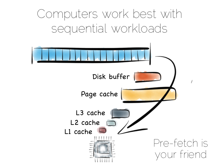
In a somewhat abstract sense, when we’re dealing with data, we’re really just arranging locality. Locality to the CPU. Locality to the other data we need. Accessing data sequentially is an important component of this. Computers are just good at sequential operations. Sequential operations can be predicted.

If you’re taking data from disk sequentially it’ll be pre-fetched into the disk buffer, the page cache and the different levels of CPU caching. This has a significant effect on performance. But it does little to help the addressing of data at random, be it in main memory, on disk or over the network. In fact pre-fetching actually hinders random workloads as the various caches and frontside bus fill with data which is unlikely to be used.

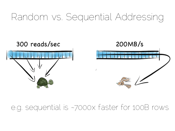
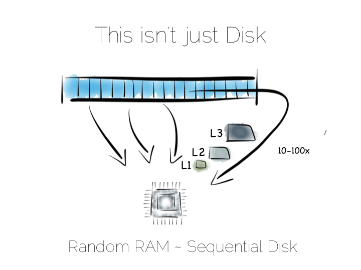
So whilst disk is somewhat renowned for its slow performance, main memory is often assumed to simply be fast. This is not as ubiquitously true as people often think. There are one to two orders of magnitude between random and sequential main memory workloads. Use a language that manages memory for you and things generally get a whole lot worse.

Streaming data sequentially from disk can actually outperform randomly addressed main memory. So disk may not always be quite the tortoise we think it is, at least not if we can arrange sequential access. SSD’s, particularly those that utilise PCIe, further complicate the picture as they demonstrate different tradeoffs, but the caching benefits of the two access patterns remain, regardless.

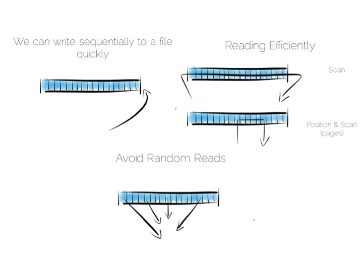
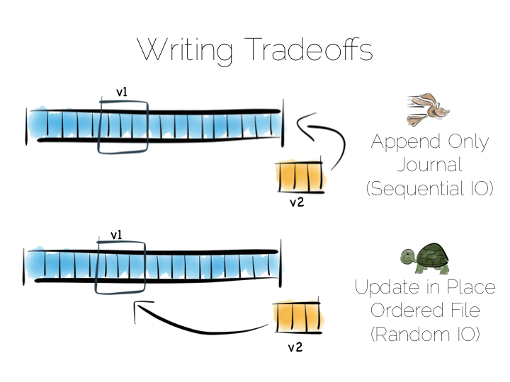
So lets imagine, as a simple thought experiment, that we want to create a very simple database. We’ll start with the basics: a file.

We want to keep writes and reads sequential, as it works well with the hardware. We can append writes to the end of the file efficiently. We can read by scanning the the file in its entirety. Any processing we wish to do can happen as the data streams through the CPU. We might filter, aggregate or even do something more complex. The world is our oyster!

So what about data that changes, updates etc?

We have a couple of options. We could update the value in place. We’d need to use fixed width fields for this, but that’s ok for our little thought experiment. But update in place would mean random IO. We know that’s not good for performance.

Alternatively we could just append updates to the end of the file and deal with the superseded values when we read it back.

So we have our first tradeoff. Append to a ‘journal’ or ‘log’, and reap the benefits of sequential access. Alternatively if we use update in place we’ll be back to 300 or so writes per second, assuming we actually flush through to the underlying media.

Now in practice of course reading the file, in its entirety, can be pretty slow. We’ll only need to get into GB’s of data and the fastest disks will take seconds. This is what a database does when it ends up table scanning.

Also we often want something more specific, say customers named “bob”, so scanning the whole file would be overkill. We need an index.

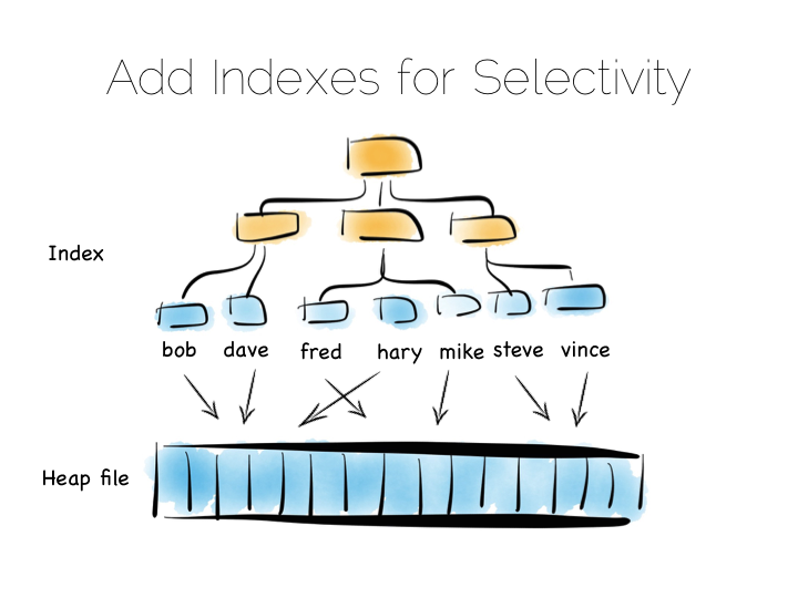
Now there are lots of different types of indexes we could use. The simplest would be an ordered array of fixed-width values, in this case customer names, held with the corresponding offsets in the heap file. The ordered array could be searched with binary search. We could also of course use some form of tree, bitmap index, hash index, term index etc. Here we’re picturing a tree.

The thing with indexes like this is that they impose an overarching structure. The values are deliberately ordered so we can access them quickly when we want to do a read. The problem with the overarching structure is that it necessitates random writes as data flows in. So our wonderful, write optimised, append only file must be augmented by writes that scatter-gun the filesystem. This is going to slow us down.

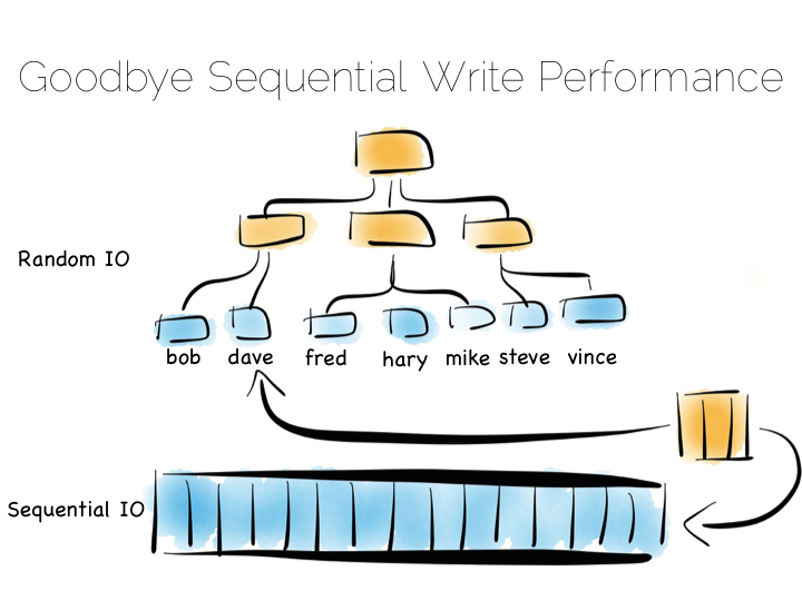
Anyone who has put lots of indexes on a database table will be familiar with this problem. If we are using a regular rotating hard drive, we might run 1,000s of times slower if we maintain disk integrity of an index in this way.

Luckily there are a few ways around this problem. Here we are going to discuss three. These represent three extremes, and they are in truth simplifications of the real world, but the concepts are useful when we consider larger compositions.

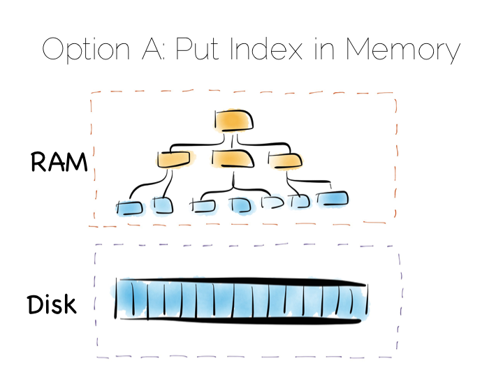
Our first option is simply to place the index in main memory. This will compartmentalise the problem of random writes to RAM. The heap file stays on disk.

This is a simple and effective solution to our random writes problem. It is also one used by many real databases. MongoDB, Cassandra, Riak and many others use this type of optimisation. Often memory mapped files are used.

However, this strategy breaks down if we have far more data than we have main memory. This is particularly noticeable where there are lots of small objects. Our index would get very large. Thus our storage becomes bounded by the amount of main memory we have available. For many tasks this is fine, but if we have very large quantities of data this can be a burden.

A popular solution is to move away from having a single ‘overarching’ index. Instead we use a collection of smaller ones.

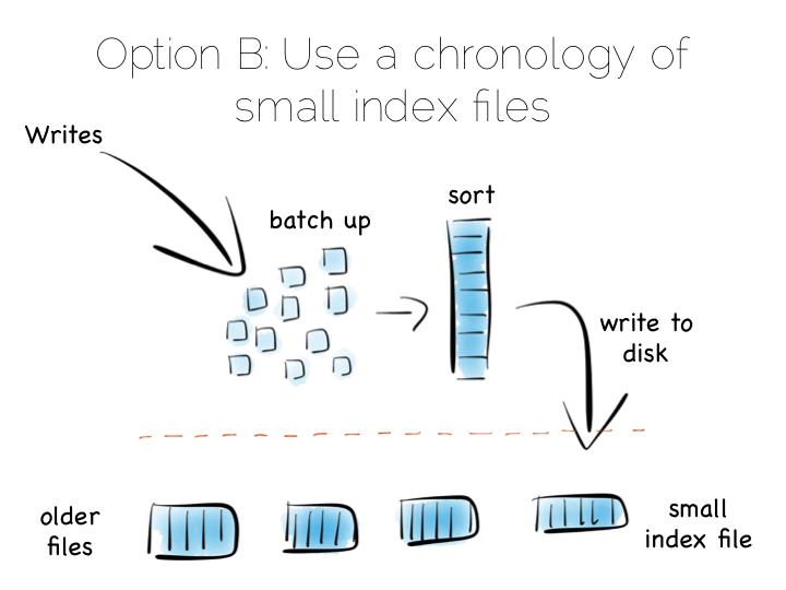
This is a simple idea. We batch up writes in main memory, as they come in. Once we have sufficient – say a few MB’s – we sort them and write them to disk as an individual mini-index. What we end up with is a chronology of small, immutable index files.

So what was the point of doing that? Our set of immutable files can be streamed sequentially. This brings us back to a world of fast writes, without us needing to keep the whole index in memory. Nice!

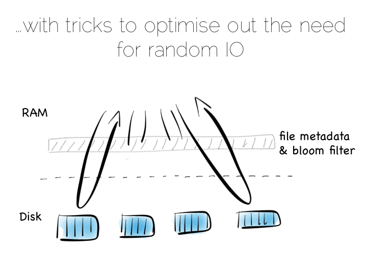
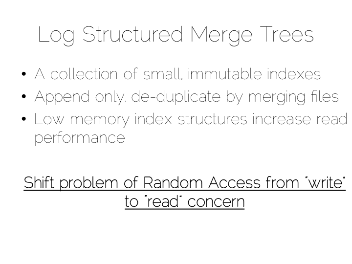
Of course there is a downside to this approach too. When we read, we have to consult the many small indexes individually. So all we have really done is shift the problem of RandomIO from writes onto reads. However this turns out to be a pretty good tradeoff in many cases. It’s easier to optimise random reads than it is to optimise random writes.

Keeping a small meta-index in memory or using a Bloom Filter provides a low-memory way of evaluating whether individual index files need to be consulted during a read operation. This gives us almost the same read performance as we’d get with a single overarching index whilst retaining fast, sequential writes.

In reality we will need to purge orphaned updates occasionally too, but that can be done with nice sequential reads and writes.

What we have created is termed a Log Structured Merge Tree. A storage approach used in a lot of big data tools such as HBase, Cassandra, Google’s BigTable and many others. It balances write and read performance with comparatively small memory overhead.

So we can get around the ‘random-write penalty’ by storing our indexes in memory or, alternatively, using a write-optimised index structure like LSM. There is a third approach though. Pure brute force.

Think back to our original example of the file. We could read it in its entirety. This gave us many options in terms of how we go about processing the data within it. The brute force approach is simply to hold data by column rather than by row. This approach is termed Columnar or Column Oriented.

(It should be noted that there is an unfortunate nomenclature clash between true column stores and those that follow the Big Table pattern. Whilst they share some similarities, in practice they are quite different. It is wise to consider them as different things.)

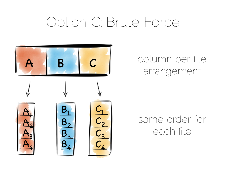
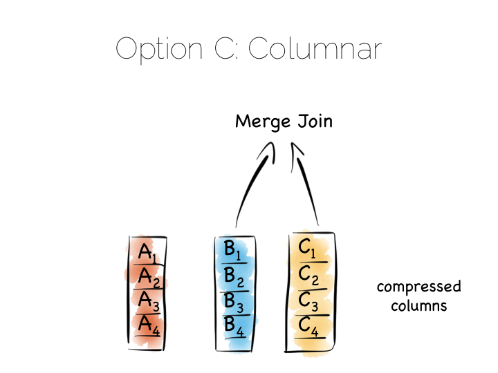
Column Orientation is another simple idea. Instead of storing data as a set of rows, appended to a single file, we split each row by column. We then store each column in a separate file. When we read we only read the columns we need.

We keep the order of the files the same, so row N has the same position (offset) in each column file. This is important because we will need to read multiple columns to service a single query, all at the same time. This means ‘joining’ columns on the fly. If the columns are in the same order we can do this in a tight loop which is very cache- and cpu-efficient. Many implementations make heavy use of vectorisation to further optimise throughput for simple join and filter operations.

Writes can leverage the benefits of being append-only. The downside is that we now have many files to update, one for every column in every individual write to the database. The most common solution to this is to batch writes in a similar way to the one used in the LSM approach above. Many columnar databases also impose an overall order to the table as a whole to increase their read performance for one chosen key.

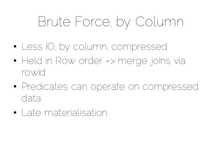
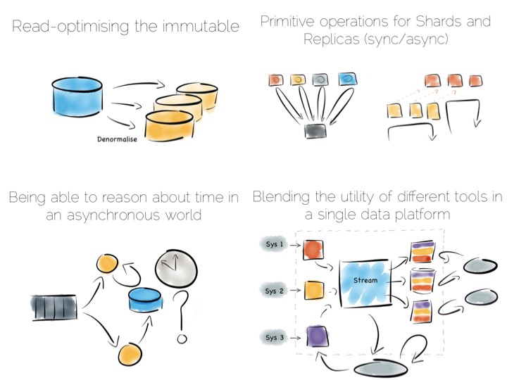
By splitting data by column we significantly reduce the amount of data that needs to be brought from disk, so long as our query operates on a subset of all columns.

In addition to this, data in a single column generally compresses well. We can take advantage of the data type of the column to do this, if we have knowledge of it. This means we can often use efficient, low cost encodings such as run-length, delta, bit-packed etc. For some encodings predicates can be used directly on the compressed stream too.

The result is a brute force approach that will work particularly well for operations that require large scans. Aggregate functions like average, max, min, group by etc are typical of this.

This is very different to using the ‘heap file & index’ approach we covered earlier. A good way to understand this is to ask yourself: what is the difference between a columnar approach like this vs a ‘heap & index’ where indexes are added to every field?

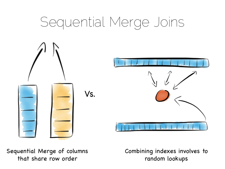
The answer to this lies in the ordering of the index files. BTrees etc will be ordered by the fields they index. Joining the data in two indexes involves a streaming operation on one side, but on the other side the index lookups have to read random positions in the second index. This is generally less efficient than joining two indexes (columns) that retain the same ordering. Again we’re leveraging sequential access.

So many of the best technologies which we may want to use as components in a data platform will leverage one of these core efficiencies to excel for a certain set of workloads.

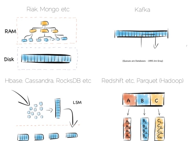
Storing indexes in memory, over a heap file, is favoured by many NoSQL stores such as Riak, Couchbase or MongoDB as well as some relational databases. It’s a simple model that works well.

Tools designed to work with larger data sets tend to take the LSM approach. This gives them fast ingestion as well as good read performance using disk based structures. HBase, Cassandra, RocksDB, LevelDB and even Mongo now support this approach.

Column-per-file engines are used heavily in MPP databases like Redshift or Vertica as well as in the Hadoop stack using Parquet. These are engines for data crunching problems that require large traversals. Aggregation is the home ground for these tools.

Other products like Kafka apply the use of a simple, hardware efficient contract to messaging. Messaging, at its simplest, is just appending to a file, or reading from a predefined offset. You read messages from an offset. You go away. You come back. You read from the offset you previously finished at. All nice sequential IO.

This is different to most message oriented middleware. Specifications like JMS and AMQP require the addition of indexes like the ones discussed above, to manage selectors and session information. This means they often end up performing more like a database than a file. Jim Gray made this point famously back in his 1995 publication Queue’s are Databases.

So all these approaches favour one tradeoff or other, often keeping things simple, and hardware sympathetic, as a means of scaling.

So we’ve covered some of the core approaches to storage engines. In truth we made some simplifications. The real world is a little more complex. But the concepts are useful nonetheless.

Scaling a data platform is more than just storage engines though. We need to consider parallelism.

When distributing data over many machines we have two core primitives to play with: partitioning and replication. Partitioning, sometimes called sharding, works well both for random access and brute force workloads.

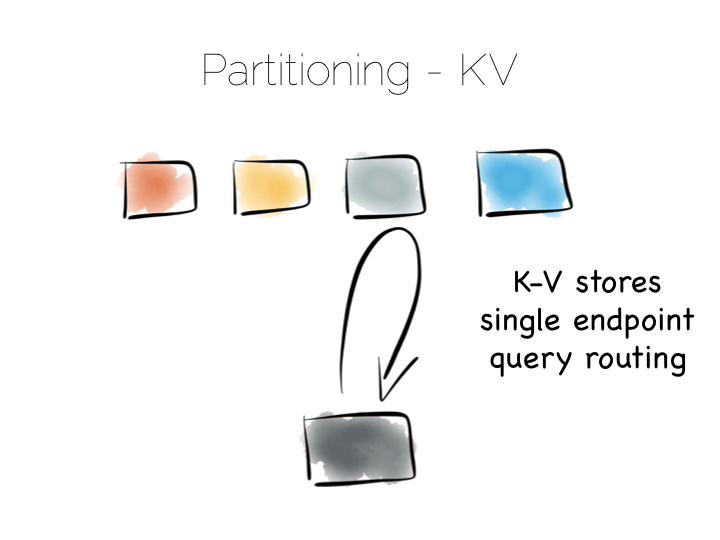
If a hash-based partitioning model is used the data will be spread across a number of machines using a well-known hash function. This is similar to the way a hash table works, with each bucket being held on a different machine.

The result is that any value can be read by going directly to the machine that contains the data, via the hash function. This pattern is wonderfully scalable and is the only pattern that shows linear scalability as the number of client requests increases. Requests are isolated to a single machine. Each one will be served by just a single machine in the cluster.

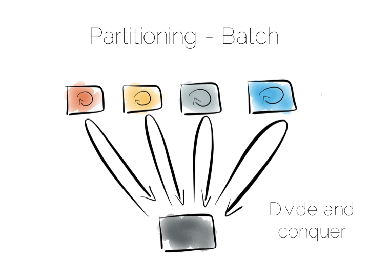
We can also use partitioning to provide parallelism over batch computations, for example aggregate functions or more complex algorithms such as those we might use for clustering or machine learning. The key difference is that we exercise all machines at the same time, in a broadcast manner. This allows us to solve a large computational problem in a much shorter time, using a divide and conquer approach.

Batch systems work well for large problems, but provide little concurrency as they tend to exhaust the resources on the cluster when they execute.

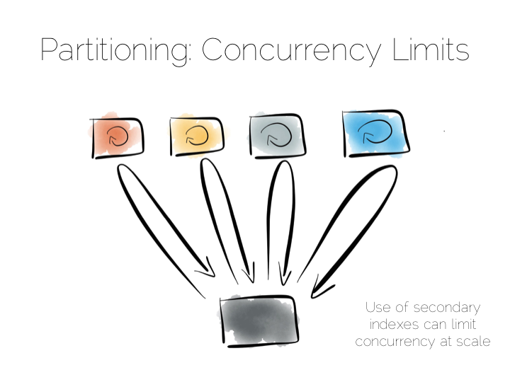
So the two extremes are pretty simple: Directed access at one end. Broadcast, divide and conquer at the other. Where we need to be careful is in the middle ground that lies between the two. A good example of this is the use of secondary indexes in NoSQL stores that span many machines.

A secondary index is an index that isn’t on the primary key. This means the data will not be partitioned by the values in the index. Directed routing via a hash function is no longer an option. We have to broadcast requests to all machines. This limits concurrency. Every node must be involved in every query.

For this reason many key value stores have resisted the temptation to add secondary indexes, despite their obvious use. HBase and Voldemort are examples of this. But many others do expose them, MongoDB, Cassandra, Riak etc. This is good as secondary indexes are useful. But it’s important to understand the effect they will have on the overall concurrency of the system.

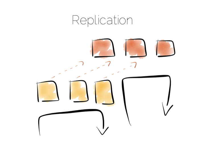
The route out of this concurrency bottleneck is replication. You’ll probably be familiar with replication either from using async slave databases or from replicated NoSQL stores like Mongo or Cassandra.

In practice replicas can be invisible (used only for recovery), read only (adding concurrency) or read-write (adding availability under network partitions). Which of these you choose will trade off against the consistency of the system. This is simply the application of CAP theorem (although cap theorem also may not be as simple as you think).

This tradeoff with consistency* brings us to an important question. When does consistency matter?

Consistency is expensive. In the database world ACID is guaranteed by linearisabilty. This is essentially ensuring that all operations appear to occur in sequential order. It turns out to be a pretty expensive thing. In fact it’s prohibitive enough that many databases don’t offer it as an isolation level at all. Those that do, rarely set it as the default.

Suffice to say that if you apply strong consistency to a system that does distributed writes you’ll likely end up in tortoise territory.

(* note the term consistency has two common usages. The C in ACID and the C in CAP. They are unfortunately not the same. I’m using the CAP definition: all nodes see the same data at the same time)

The solution to this consistency problem is simple. Avoid it. If you can’t avoid it isolate it to as few writers and as few machines as possible.

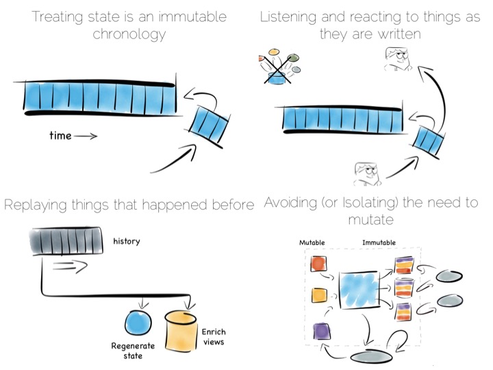
Avoiding consistency issues is often quite easy, particularly if your data is an immutable stream of facts. A set of web logs is a good example. They have no consistency concerns as they are just facts that never change.

There are other use cases which do necessitate consistency though. Transferring money between accounts is an oft used example. Non-commutative actions such as applying discount codes is another.

But often things that appear to need consistency, in a traditional sense, may not. For example if an action can be changed from a mutation to a new set of associated facts we can avoid mutable state. Consider marking a transaction as being potentially fraudulent. We could update it directly with the new field. Alternatively we could simply use a separate stream of facts that links back to the original transaction.

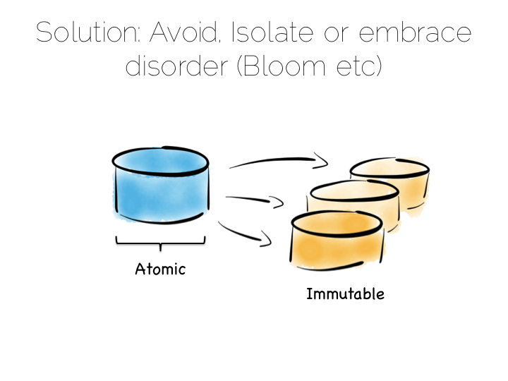
So in a data platform it’s useful to either remove the consistency requirement altogether, or at least isolate it. One way to isolate is to use the single writer principal, this gets you some of the way. Datomic is a good example of this. Another is to physically isolate the consistency requirement by splitting mutable and immutable worlds.

Approaches like Bloom/CALM extend this idea further by embracing the concept of disorder by default, imposing order only when necessary.

So those were some of the fundamental tradeoffs we need to consider. Now how to we pull these things together to build a data platform?

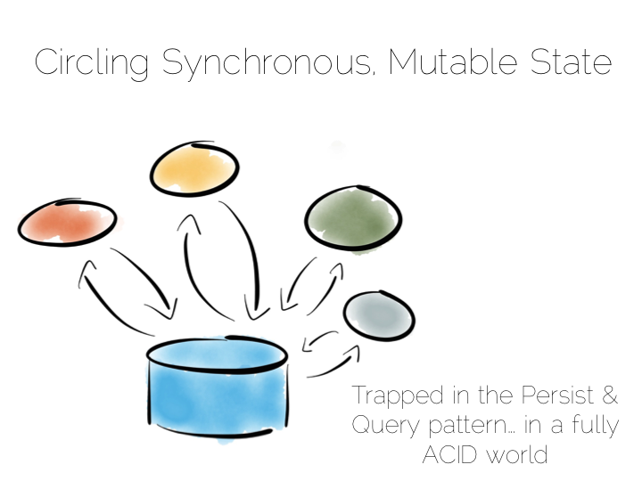
A typical application architecture might look something like the below. We have a set of processes which write data to a database and read it back again. This is fine for many simple workloads. Many successful applications have been built with this pattern. But we know it works less well as throughput grows. In the application space this is a problem we might tackle with message-passing, actors, load balancing etc.

The other problem is this approach treats the database as a black box. Databases are clever software. They provide a huge wealth of features. But they provide few mechanisms for scaling out of an ACID world. This is a good thing in many ways. We default to safety. But it can become an annoyance when scaling is inhibited by general guarantees which may be overkill for the requirements we have.

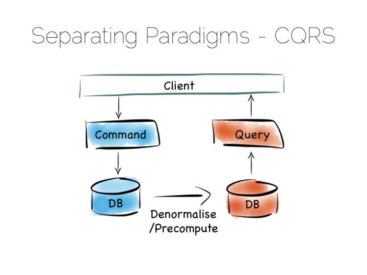
The simplest route out of this is CQRS (Command Query Responsibility Segregation).

Another very simple idea. We separate read and write workloads. Writes go into something write-optimised. Something closer to a simple journal file. Reads come from something read-optimised. There are many ways to do this, be it tools like Goldengate for relational technologies or products that integrate replication internally such as Replica Sets in MongoDB.

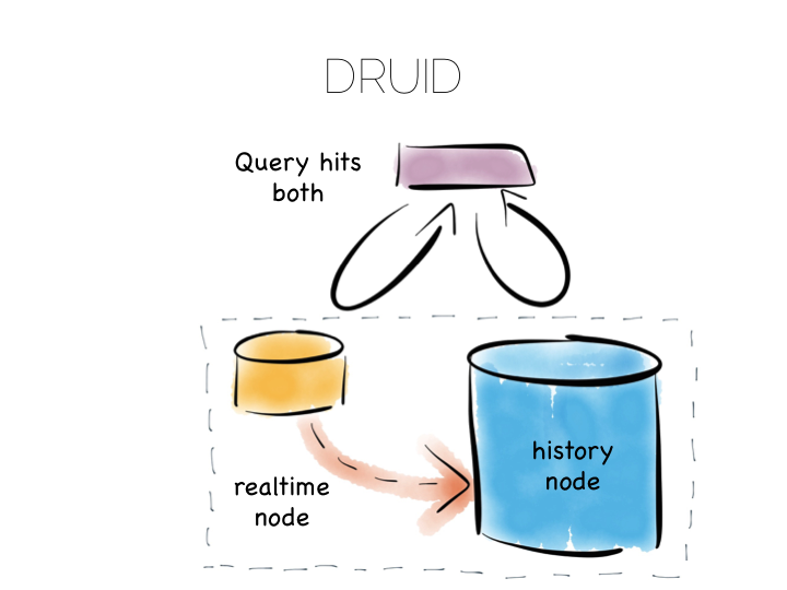
Many databases do something like this under the hood. Druid is a nice example. Druid is an open source, distributed, time-series, columnar analytics engine. Columnar storage works best if we input data in large blocks, as the data must be spread across many files. To get good write performance Druid stores recent data in a write optimised store. This is gradually ported over to the read optimised store over time.

When Druid is queried the query routes to both the write optimised and read optimised components. The results are combined (‘reduced’) and returned to the user. Druid uses time, marked on each record, to determine ordering.

Composite approaches like this provide the benefits of CQRS behind a single abstraction.

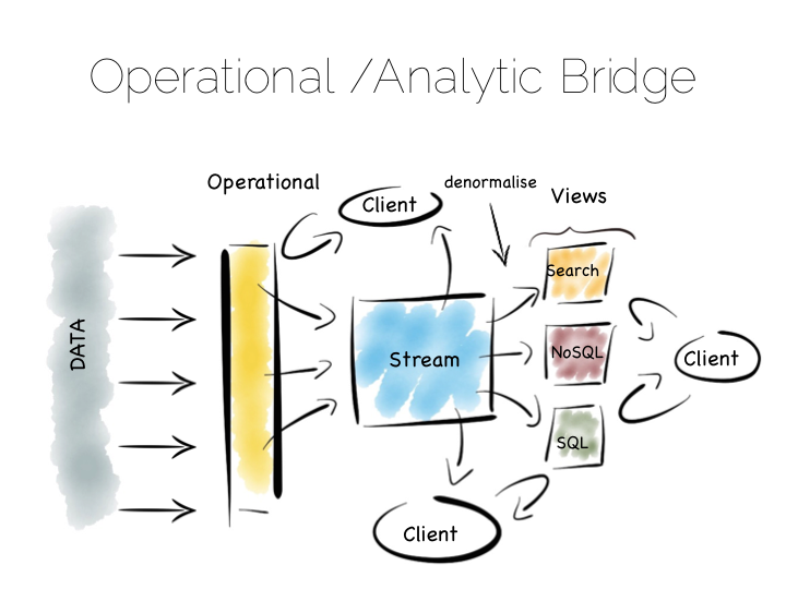
Another similar approach is to use an Operational/Analytic Bridge. Read- and write-optimised views are separated using an event stream. The stream of state is retained indefinitely, so that the async views can be recomposed and augmented at a later date by replaying.

So the front section provides for synchronous reads and writes. This can be as simple as immediately reading data that was written or as complex as supporting ACID transactions.

The back end leverages asynchronicity, and the advantages of immutable state, to scale offline processing through replication, denormalisation or even completely different storage engines. The messaging-bridge, along with joining the two, allows applications to listen to the data flowing through the platform.

As a pattern this is well suited to mid-sized deployments where there is at least a partial, unavoidable requirement for a mutable view.

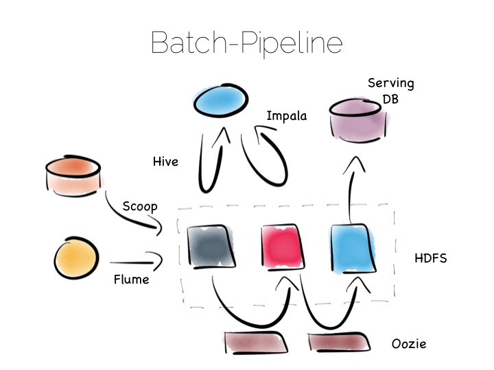
If we are designing for an immutable world, it’s easier to embrace larger data sets and more complex analytics. The batch pipeline, one almost ubiquitously implemented with the Hadoop stack, is typical of this.

The beauty of the Hadoop stack comes from it’s plethora of tools. Whether you want fast read-write access, cheap storage, batch processing, high throughput messaging or tools for extracting, processing and analysing data, the Hadoop ecosystem has it all.

The batch pipeline architecture pulls data from pretty much any source, push or pull. Ingests it into HDFS then processes it to provide increasingly optimised versions of the original data. Data might be enriched, cleansed, denormalised, aggregated, moved to a read optimised format such as Parquet or loaded into a serving layer or data mart. Data can be queried and processed throughout this process.

This architecture works well for immutable data, ingested and processed in large volume. Think 100’s of TBs (although size alone isn’t a great metric). The evolution of this architecture will be slow though. Straight-through timings are often measured in hours.

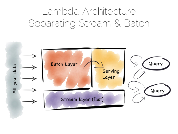
The problem with the Batch Pipeline is that we often don’t want to wait hours to get a result. A common solution is to add a streaming layer aside it. This is sometimes referred to as the Lambda Architecture.

The Lambda Architecture retains a batch pipeline, like the one above, but it circumvents it with a fast streaming layer. It’s a bit like building a bypass around a busy town. The streaming layer typically uses a streaming processing tool such as Storm or Samza.

The key insight of the Lambda Architecture is that we’re often happy to have an approximate answer quickly, but we would like an accurate answer in the end.

So the streaming layer bypasses the batch layer providing the best answers it can within a streaming window. These are written to a serving layer. Later the batch pipeline computes an accurate data and overwrites the approximation.

This is a clever way to balance accuracy with responsiveness. Some implementations of this pattern suffer if the two branches end up being dual coded in stream and batch layers. But it is often possible to simply abstract this logic into common libraries that can be reused, particularly as much of this processing is often written in external libraries such as Python or R anyway. Alternatively systems like Spark provide both stream and batch functionality in one system (although the streams in Spark are really micro-batches).

So this pattern again suits high volume data platforms, say in the 100TB range, that want to combine streams with existing, rich, batch based analytic function.

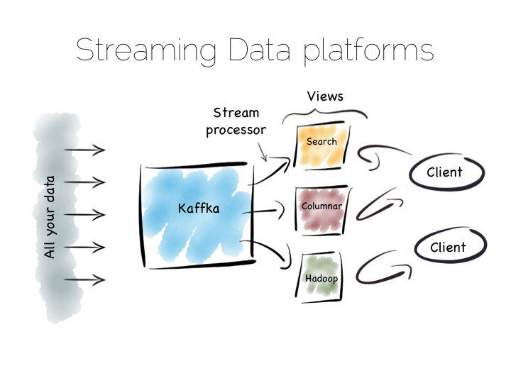
There is another approach to this problem of slow data pipelines. It’s sometimes termed the Kappa architecture. I actually thought this name was ‘tongue in cheek’ but I’m now not so sure. Whichever it is, I’m going to use the term Stream Data Platform, which is a term in use also.

Stream Data Platform’s flip the batch pattern on its head. Rather than storing data in HDFS, and refining it with incremental batch jobs, the data is stored in a scale out messaging system, or log, such as Kafka. This becomes the system of record and the stream of data is processed in real time to create a set of tertiary views, indexes, serving layers or data marts.

This is broadly similar to the streaming layer of the Lambda architecture but with the batch layer removed. Obviously the requirement for this is that the messaging layer can store and vend very large volumes of data and there is a sufficiently powerful stream processor to handle the processing.

There is no free lunch so, for hard problems, Stream Data Platform’s will likely run no faster than an equivalent batch system, but switching the default approach from ‘store and process’ to ‘stream and process’ can provide greater opportunity for faster results.

Finally, the Stream Data Platform approach can be applied to the problem of ‘application integration’. This is a thorny and difficult problem that has seen focus from big vendors such as Informatica, Tibco and Oracle for many years. For the most part results have been beneficial, but not transformative. Application integration remains a topic looking for a real workable solution.

Stream Data Platform’s provide an interesting potential solution to this problem. They take many of the benefits of an O/A bridge – the variety of asynchronous storage formats and ability to recreate views – but leave the consistency requirement isolated in, often existing sources:

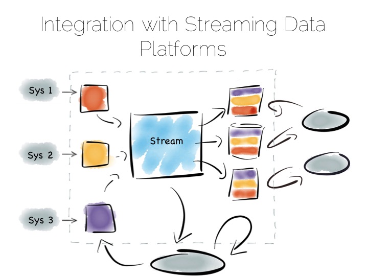
With the system of record being a log it’s easy to enforce immutability. Products like Kafka can retain enough volume and throughput, internally, to be used as a historic record. This means recovery can be a process of replaying and regenerating state, rather than constantly checkpointing.

Similarly styled approaches have been taken before in a number of large institutions with tools such as Goldengate, porting data to enterprise data warehouses or more recently data lakes. They were often thwarted by a lack of throughput in the replication layer and the complexity of managing changing schemas. It seems unlikely the first problem will continue. As for the later problem though, the jury is still out.

So we started with locality. With sequential addressing for both reads and writes. This dominates the tradeoffs inside the components we use. We looked at scaling these components out, leveraging primitives for both sharding and replication. Finally we rebranded consistency as a problem we should isolate in the platforms we build.

But data platforms themselves are really about balancing the sweet-spots of these individual components within a single, holistic form. Incrementally restructuring. Migrating the write-optimised to the read-optimised. Moving from the constraints of consistency to the open plains of streamed, asynchronous, immutable state.

This must be done with a few things in mind. Schemas are one. Time, the peril of the distributed, asynchronous world, is another. But these problems are manageable if carefully addressed. Certainly the future is likely to include more of these things, particularly as tooling, innovated in the big data space, percolates into platforms that address broader problems, both old and new.

THINGS WE LIKE

Follow @Benstopford

Posted in Analysis and Opinion, Blog, Talks, Top4 | 19 Comments »

Log Structured Merge Trees

Saturday, February 14th, 2015

It’s nearly a decade since Google released its ‘Big Table’ paper. One of the many cool aspects of that paper was the file organisation it uses. The approach is more generally known as the Log Structured Merge Tree, after this 1996 paper, although the algorithm described there differs quite significantly from most real-world implementations.

LSM is now used in a number of products as the main file organisation strategy. HBase, Cassandra, LevelDB, SQLite, even MongoDB 3.0 comes with an optional LSM engine, after it’s acquisition of Wired Tiger.

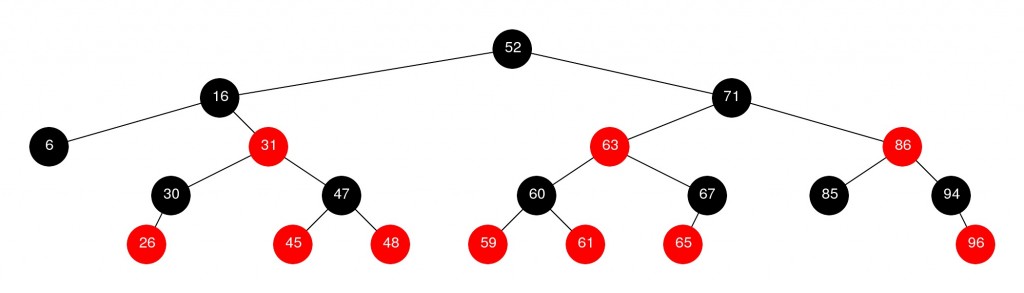
What makes LSM trees interesting is their departure from binary tree style file organisations that have dominated the space for decades. LSM seems almost counter intuitive when you first look at it, only making sense when you closely consider how files work in modern, memory heavy systems.

Some Background

In a nutshell LSM trees are designed to provide better write throughput than traditional B+ tree or ISAM approaches. They do this by removing the need to perform dispersed, update-in-place operations.

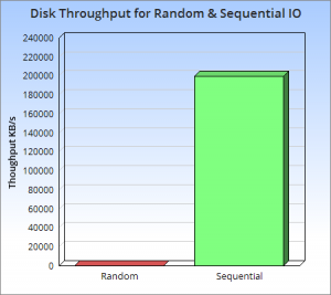ChartGo So why is this a good idea? At its core it’s the old problem of disks being slow for random operations, but fast when accessed sequentially. A gulf exists between these two types of access, regardless of whether the disk is magnetic or solid state or even, although to a lesser extent, main memory.

The figures in this ACM report here/here make the point well. They show that, somewhat counter intuitively, sequential disk access is faster than randomly accessing main memory. More relevantly they also show sequential access to disk, be it magnetic or SSD, to be at least three orders of magnitude faster than random IO. This means random operations are to be avoided. Sequential access is well worth designing for.

So with this in mind lets consider a little thought experiment: if we are interested in write throughput, what is the best method to use? A good starting point is to simply append data to a file. This approach, often termed logging, journaling or a heap file, is fully sequential so provides very fast write performance equivalent to theoretical disk speeds (typically 200-300MB/s per drive).

Benefiting from both simplicity and performance log/journal based approaches have rightfully become popular in many big data tools. Yet they have an obvious downside. Reading arbitrary data from a log will be far more time consuming than writing to it, involving a reverse chronological scan, until the required key is found.

This means logs are only really applicable to simple workloads, where data is either accessed in its entirety, as in the write-ahead log of most databases, or by a known offset, as in simple messaging products like Kafka.

So we need more than just a journal to efficiently perform more complex read workloads like key based access or a range search. Broadly speaking there are four approaches that can help us here: binary search, hash, B+ or external.

Search Sorted File: save data to a file, sorted by key. If data has defined widths use Binary search. If not use a page index + scan.
Hash: split the data into buckets using a hash function, which can later be used to direct reads.
B+: use navigable file organisation such as a B+ tree, ISAM etc.
External file: leave the data as a log/heap and create a separate hash or tree index into it.

All these approaches improve read performance significantly ( n->O(log(n)) in most). Alas these structures add order and that order impedes write performance, so our high speed journal file is lost along the way. You can’t have your cake and eat it I guess.

tree (2)

An insight that is worth making is that all four of the above options impose some form of overarching structure on the data.

Data is deliberately and specifically placed around the file system so the index can quickly find it again later. It’s this structure that makes navigation quick. Alas the structure must of course be honoured as data is written. This is where we start to degrade write performance by adding in random disk access.

There are a couple of specific issues. Two IOs are needed for each write, one to read the page and one to write it back. This wasn’t the case with our log/journal file which could do it in one.

Worse though, we now need to update the structure of the hash or B+ index. This means updating specific parts of the file system. This is known as update-in-place and requires slow, random IO. This point is important: in-place approaches like this scatter-gun the file system performing update-in-place*. This is limiting.

One common solution is to use approach (4) A index into a journal – but keep the index in memory. So, for example, a Hash Table can be used to map keys to the position (offset) of the latest value in a journal file (log). This approach actually works pretty well as it compartmentalises random IO to something relatively small: the key-to-offset mapping, held in memory. Looking up a value is then only a single IO.

On the other hand there are scalability limits, particularly if you have lots of small values. If your values were just say simple numbers then the index would be larger than the data file itself. Despite this the pattern is a sensible compromise which is used in many products from Riak through to Oracle Coherence.

So this brings us on to Log Structured Merge Trees. LSMs take a different approach to the four above. They can be fully disk-centric, requiring little in memory storage for efficiency, but also hang onto much of the write performance we would tie to a simple journal file. The one downside is slightly poorer read performance when compared to say a B+Tree.

In essence they do everything they can to make disk access sequential. No scatter-guns here!

*A number of tree structures exist which do not require update-in-place. Most popular is the append-only Btree, also know as the copy-on-write tree. These work by overwriting the tree structure, sequentially, at the end of the file each time a write occurs. Relevant parts of the old tree structure, including the top level node, are orphaned. Through this method update-in-place is avoided as the tree sequentially redefines itself over time. This method does however come at the cost: rewriting the structure on every write is verbose. It creates a significant amount of write amplification which is a downside unto itself.

The Base LSM Algorithm

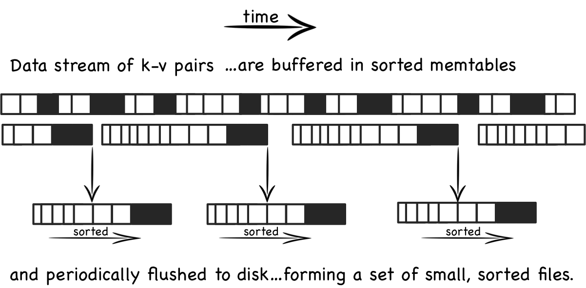
Conceptually the base LSM tree is fairly simple. Instead of having one big index structure (which will either scatter-gun the file system or add significant write amplification) batches of writes are saved, sequentially, to a set of smaller index files. So each file contains a batch of changes covering a short period of time. Each file is sorted before it is written so searching it later will be fast. Files are immutable; they are never updated. New updates go into new files. Reads inspect all files. Periodically files are merged together to keep the number of files down.

Lets look at this in a little more detail. When updates arrive they are added to an in-memory buffer, which is usually held as a tree (Red-Black etc) to preserve key-ordering. This ‘memtable’ is replicated on disk as a write-ahead-log in most implementations, simply for recovery purposes. When the memtable fills the sorted data is flushed to a new file on disk. This process repeats as more and more writes come in. Importantly the system is only doing sequential IO as files are not edited. New entries or edits simply create successive files (see fig above).

So as more data comes into the system, more and more of these immutable, ordered files are created. Each one representing a small, chronological subset of changes, held sorted.

As old files are not updated duplicate entries are created to supersede previous records (or removal markers). This creates some redundancy initially.

Periodically the system performs a compaction. Compaction selects multiple files and merges them together, removing any duplicated updates or deletions (more on how this works later). This is important both to remove the aforementioned redundancy but, more importantly, to keep a handle on the read performance which degrades as the number of files increases. Thankfully, because the files are sorted, the process of merging the files is quite efficient.

When a read operation is requested the system first checks the in memory buffer (memtable). If the key is not found the various files will be inspected one by one, in reverse chronological order, until the key is found. Each file is held sorted so it is navigable. However reads will become slower and slower as the number of files increases, as each one needs to be inspected. This is a problem.

So reads in LSM trees are slower than their in-place brethren. Fortunately there are a couple of tricks which can make the pattern performant. The most common approach is to hold a page-index in memory. This provides a lookup which gets you ‘close’ to your target key. You scan from there as the data is sorted. LevelDB, RocksDB and BigTable do this with a block-index held at the end of each file. This often works better than straight binary search as it allows the use of variable length fields and is better suited to compressed data.

Even with per-file indexes read operations will still slow as the number of files increases. This is kept in check by periodically merging files together. Such compactions keep the number of files, and hence read performance, within acceptable bounds.

Even with compaction reads will still need to visit many files. Most implementations void this through the use of a Bloom filter. Bloom filters are a memory efficient way of working out whether a file contains a key.

So from a ‘write’ perspective; all writes are batched up and written only in sequential chunks. There is an additional, periodic IO penalty from compaction rounds. Reads however have the potential to touch a large number of files when looking up a single row (i.e. scatter-gun on read). This is simply the way the algorithm works. We’re trading random IO on write for random IO on read. This trade off is sensible if we can use software tricks like bloom filters or hardware tricks like large file caches to optimise read performance.

Basic Compaction

To keep LSM reads relatively fast it’s important to manage-down the number of files, so lets look more deeply at compaction. The process is a bit like generational garbage collection:

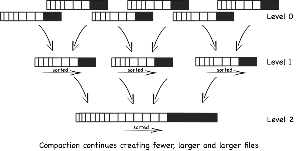
When a certain number of files have been created, say five files, each with 10 rows, they are merged into a single file, with 50 rows (or maybe slightly less) .

This process continues with more 10 row files being created. These are merged into 50 row files every time the fifth file fills up.

Eventually there are five 50 row files. At this point the five 50 row files are merged into one 250 row file. The process continues creating larger and larger files. See fig.

The aforementioned issue with this general approach is the large number of files that are created: all must be searched, individually, to read a result (at least in the worst case).

Journal2.5

Levelled Compaction

Newer implementations, such as those in LevelDB, RocksDB and Cassandra, address this problem by implementing a level-based, rather than size-based, approach to compaction. This reduces the number of files that must be consulted for the worst case read, as well as reducing the relative impact of a single compaction.

This level-based approach has two key differences compared to the base approach above:

1. Each level can contain a number of files and is guaranteed, as a whole, to not have overlapping keys within it. That is to say the keys are partitioned across the available files. Thus to find a key in a certain level only one file needs to be consulted.

The first level is a special case where the above property does not hold. Keys can span multiple files.

2. Files are merged into upper levels one file at a time. As a level fills, a single file is plucked from it and merged into the level above creating space for more data to be added. This is slightly different to the base-approach where several similarly sized files are merged into a single, larger one.

These changes mean the level-based approach spreads the impact of compaction over time as well as requiring less total space. It also has better read performance. However the total IO is higher for most workloads meaning some of the simpler write-oriented workloads will not see benefit.

Summarising

So LSM trees sit in the middle-ground between a journal/log file and a traditional single-fixed-index such as a B+ tree or Hash index. They provide a mechanism for managing a set of smaller, individual index files.

By managing a group of indexes, rather than a single one, the LSM method trades the expensive random IO associated with update-in-place in B+ or Hash indexes for fast, sequential IO.

The price being paid is that reads have to address a large number of index files rather than just the one. Also there is additional IO cost for compaction.

If that’s still a little murky there are some other good descriptions here and here.

Thoughts on the LSM approach

So are LSM approaches really better than traditional single-tree based ones?

We’ve seen that LSM’s have better write performance albeit a cost. LSM has some other benefits though. The SSTables (the sorted files) a LSM tree creates are immutable. This makes the locking semantics over them much simpler. Generally the only resource that is contended is the memtable. This is in contrast to singular trees which require elaborate locking mechanisms to manage changes at different levels.

So ultimately the question is likely to be about how write-oriented expected workloads are. If you care about write performance the savings LSM gives are likely to be a big deal. The big internet companies seem pretty settled on this subject. Yahoo, for example, reports a steady progression from read-heavy to read-write workloads, driven largely by the increased ingestion of event logs and mobile data. Many traditional database products still seem to favour more read-optimised file structures though.

As with Log Structured file systems [see footnote] the key argument stems from the increasing availability of memory. With more memory available reads are naturally optimised through large file caches provided by the operating system. Write performance (which memory doesn’t improve with more) thus becomes the dominant concern. So put another way, hardware advances are doing more for read performance than they are for writes. Thus it makes sense to select a write-optimised file structure.

Certainly LSM implementations such as LevelDB and Cassandra regularly provide better write performance than single-tree based approaches (here and here respectively).

Beyond Levelled LSM

There has been a fair bit of further work building on the LSM approach. Yahoo developed a system called Pnuts which combines LSM with B trees and demonstrates better performance. I haven’t seen openly available implementations of this algorithm though. IBM and Google have done more recent work in a similar vein, albeit via a different path. There are also related approaches which have similar properties but retain an overarching structure. These include Fractal Trees and Stratified Trees.

This is of course just one alternative. Databases utilise a huge range of subtly different options. An increasing number of databases offer pluggable engines for different workloads. Parquet is a popular alternative for HDFS and pushes in pretty much the opposite direction (aggregation performance via a columnar format). MySQL has a storage abstraction which is pluggable with a number of different engines such as Toku‘s fractal tree based index. This is also available for MongoDB. Mongo 3.0 includes the Wired Tiger engine which provides both B+ & LSM approaches along with the legacy engine. Many relational databases have configurable index structures that utilise different file organisations.

It’s also worth considering the hardware being used. Expensive solid state disks, like FusionIO, have better random write performance. This suits update-in-place approaches. Cheaper SSDs and mechanical drives are better suited to LSM. LSM’s avoid the small random access patters that thrash SSDs into oblivion**.

LSM is not without it critics though. It’s biggest problem, like GC, is the collection phases and the effect they have on precious IO. There is an interesting discussion of some of these on this hacker news thread.

So if you’re looking at data products, be it BDB vs. LevelDb, Cassandra vs. MongoDb you may tie some proportion of their relative performance back to the file structures they use. Measurements appear to back this philosophy. Certainly it’s worth being aware of the performance tradeoffs being selected by the systems you use.

**In SSDs each write incurs a clear-rewrite cycle for a whole 512K block. Thus small writes can induce a disproportionate amount of churn on the drive. With fixed limits on block rewrites this can significantly affect their life.

Footnote on log structured file systems

Other than the name, and a focus on write throughput, there isn’t that much relation between LSM and log structured file systems as far as I can see.

Regular filesystems used today tend to be ‘Journaling’, for example ext3, ext4, HFS etc are tree-based approaches. A fixed height tree of inodes represent the directory structure and a journal is used to protect against failure conditions. In these implementations the journal is logical, meaning it only internal metadata will be journaled. This is for performance reasons.

Log structured file systems are widely used on flash media as they have less write amplification. They are getting more press too as file caching starts to dominate read workloads in more general situations and write performance is becoming more critical.

In log structured file systems data is written only once, directly to a journal which is represented as a chronologically advancing buffer. The buffer is garbage collected periodically to remove redundant writes. Like LSM’s the log structured file system will write faster, but read slower than its dual-writing, tree based counterpart. Again this is acceptable where there is lots of RAM available to feed the file cache or the media doesn’t deal well with update in place, as is the case with flash.

Posted in Analysis and Opinion, Big Data, Blog, Top4 | 16 Comments »

ben stopford

‘Top4’

Book: Designing Event Driven Systems

The Data Dichotomy

Elements of Scale: Composing and Scaling Data Platforms

Log Structured Merge Trees

Some Background

The Base LSM Algorithm

Basic Compaction

Levelled Compaction

Summarising

Thoughts on the LSM approach

Beyond Levelled LSM

Further Reading

Footnote on log structured file systems

ALL

Talks (View on YouTube)

Essays (all)

Test Driven Development (all)

Coherence (all)

About

Data Tech (all)

Team / Process / Interviewing (all)