‘Coherence’
The Fallacy of Linear Scalability
Saturday, December 12th, 2009
The underpinning of Shared Nothing data stores is that adding a machine to a cluster proportionally increases the amount of CPU, network bandwidth and storage available. This is, of course, a fact, however the statement is only really of value if the mechanism used for reading and writing data also scales linearly, with respect to each of these physical resources.
A typical Key-Value access pattern works well: store.put(key, val), store.get(key) scale linearly as the number of nodes in the cluster is increased. This scaling leverages the fact that data is sharded (spread) across the available machines. Any single read or write operation is simply routed to the machine that owns the partition i.e. only one machine is ever asked to service a single ‘get’.
The problem is that, in real world use cases, ‘get’ and ‘put’ are often not enough and data stores offer richer query interfaces. This leads users to inevitably more complex access patterns that necessitate the use of queries that do not access data via the primary key. The rub is that these queries don’t scale in the same way.
The efficiency of a K-V lookups comes from the hashing algorithm determining which machine the required value resides on. However when we query via an index there is no such optimisation to be made. Thus the query must be broadcast to all nodes in the cluster. This puts an upper bound on scalability in that:
the max number of queries serviced by the system = the max number of queries serviced by each machine
The implications for scalability are fairly obvious and noticeable when such stores are run at scale. What tends to happen in practice is that one physical resource forms the bottleneck. For high data-density systems this is often disk. So if the disk in one machine can support 100 queries per second, that will be the limit of the system no matter how many nodes it has, at least where secondary indexes are used to drive queries in this broadcast way. However, if queries per second is a direct function of data volume per machine, then adding more machines will reduce the amount of data held on each. This increases the performance of the cluster by decreasing the amount of work each node needs to perform per query.
So how do you manage this problem? There are a few techniques you can use:
-
Try to use key based access instead of queries wherever possible.
-
Increase the cluster size so that the amount of data serviced by each node is reduced. This decreases the response time for each request and thus the overall load on each server. It is however somewhat expensive and wasteful.
-
Another trick is to paginate the query over the available partitions. This doesn’t address the problem directly, rather it spreads each query over a longer time frame reducing the risk of load spikes.
So be wary of overusing secondary indexes!
Shared Nothing v.s. Shared Disk Architectures: An Independent View
Tuesday, November 24th, 2009
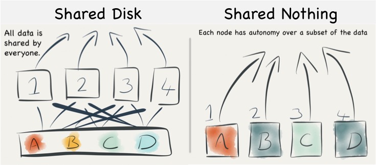
The Shared Nothing Architecture is a relatively old pattern that has had a resurgence of late in data storage technologies, particularly in the NoSQL, Data Warehousing and Big Data spaces. As architectures go it has some pretty interesting performance tradeoffs when compared to the more common approach of simply sharing a disk array (known as Shared Disk). This article compares and contrasts these two.
Shared Disk and Shared Nothing
Shared nothing is a simple idea. Data data is partitioned in some manner and spread across a set of machines. This means that each machine has sole access, and hence sole responsibility, for the data it holds. It does not share responsibility with other machines. So data is completely segregated, with each node having total autonomy over its particular subset.
By comparison shared disk is essentially the opposite: all data is accessible from all cluster nodes. Any machine can read or write any portion of data it wishes. See the figures below.
Understanding the Trade-offs for Writing
When persisting data in a shared disk architecture writes can be performed against any node. If node 1 and 2 both attempt to write a tuple then, to ensure consistency with other nodes, the management system must either use a disk based lock table or else communicated their intention to lock the tuple with the other nodes in the cluster. Both methods provide scalability issues. Adding more nodes either increases contention on the lock table or alternatively increases the number of nodes over which lock agreement must be found.
To explain this a little further consider the case described by the diagram below. The clustered shared disk database contains a record with PK = 1 and data = foo. For efficiency both nodes have cached local copies of record 1 in memory. A client then tries to update record 1 so that ‘foo’ becomes ‘bar’. To do this in a consistent manner the DBMS must take a distributed lock on all nodes that may have cached record 1. Such distributed locks become slower and slower as you increase the number of machines in the cluster and as a result can impede the scalability of the writing process.
The other mechanism, locking explicitly on disk, is rarely done in practice as caching is so fundamental to performance.
However shared nothing does not suffer from the same distributed locking problem, assuming that the client is directed to the correct node (that is to say a client writing ‘A’, in the figure above, directs that write at Node 1) , the write can flow straight though to disk with any lock mediation performed in memory. This is because only one machine has ownership of any single piece of data, hence by definition there only ever needs to be one lock.
Thus shared nothing can scale linearly from a write perspective without increasing the overhead of locking data items, because each node has sole responsibility for the data it owns.
However shared nothing will still have to execute a distributed lock for transactional writes that span data on multiple nodes (i.e. a distributed two-phase commit). These are not as large an impedance on scalability as the caching problem above, as they span only the nodes involved in the transaction (as apposed to the caching case which spans all nodes), but they add a scalability limit none the less (and they are also likely to be quite slow when compared to the shared disk case).
So shared nothing is great for systems needing high throughput writes if you can shard your data and stay clear of transactions that span different shards. The trick for this is to find the right partitioning strategy, for instance you might partition data for a online banking system such that all aspects of a user’s account are on the same machine. If the data set can be partitioned in such a way that distributed transactions are avoided then linear scalability, at least for key-based reads and writes, is at your fingertips.
The counter, from the shared disk camp, is that they can use partitioning too. Just because the disk is shared does not mean that data can’t be partitioned logically with different nodes servicing different partitions. There is much truth to this, assuming you can set up your architecture so that write requests are routed to the correct machine, as this tactic will reduce the amount of lock (or block) shipping taking place (and is exactly how you optimise databases like Oracle RAC).
Put another way – a shared disk implementation can be configured in a shared nothing mode. The difference here is just the physical placement of data. Shared disk is always network attached in some way, never local. So whilst remote disks can provide comparatively high throughput and good random IO performance they will do this at often greater monetary cost.
|
Considering the Retrieval of Data
The retrieval of data is a very different story, with different tradeoffs for each of these two approaches. Looking firstly at Shared Disk we find two significant drawbacks:
The first is the potential for resource starvation, most notably disk contention on the SAN/NAS drives. Shared disk means exactly that: all machines share the same disk array, and to some extent the same interconnect. Fortunately disk contention in a large shared disk system can be alleviated by partitioning. Data within the shared disk subsystem is often partitioned by its usage pattern (usually by moving tables onto different sections of the backing disk array). The problem with this approach is that it is manual: the data must be physically partitioned in advance.
The second issue is that caching is less efficient. Each machine in a shared disk system is likely to become involved (and hence have the requirement to cache) the whole dataset. This reduces the efficiency of the cache as cache misses are more likely. This is in stark contrast to the shared nothing approach where each machine only needs to cache the subset of the data that it owns. Thus caching can be far more effective in a shared nothing system.
Shared nothing is not without its flaws though. SN works brilliantly if the query is self sufficient – if each node can complete its ‘portion’ of the processing without needing data from any other node. However there will inevitably arise use cases where data from multiple nodes must be brought together or joined in some way. The implication is often that data, which may not be included in the final result, be shipped from one machine to another. This need to ship data between machines to ‘join’ can have a significant effect of overall query performance.
So the reality is that the number of queries requiring data shipping will depend on both the use case and the partitioning strategy. There are many cases where joins can be eliminated altogether by using Aggregates – for example in commercial search engines. However, for many general business use cases, for example ones with large related fact tables, some data shipping is often inevitable. As a result many shared nothing solutions recommend the use of fast 10GE networks.
Finally we should comment on the concurrency. Many key-value stores use shards and SN to provide very high levels of concurrency. This is achieved by routing user requests, via the sharding key, to the single machine that has the required data. This pattern is very efficient and the result is stores that provide extremely high levels of read and write throughput over a large, concurrent user base. This pattern is used heavily in large web applications via NoSQL.
What we must note is that the scalability of this pattern is only available for key-based access. It does not apply to more general processing in a shared nothing system. Any request that does not explicitly use the primary key must be broadcast to all machines (partitions). This presents a limit to the scalability for questions that do not consider the primary key. As a result many shared nothing systems, which support more general query workloads, show similar levels of concurrency to single node systems (5-10 is not uncommon).
So this is important enough to restate: Shared nothing is only linearly scalable for key-based access. The use of secondary indexes always results in every node being consulted. This limits scalability, certainly in terms of the number of concurrent requests that can be serviced. This is one of the reasons for many distributed key-value stores sticking to the very simple K-V contract.
The retort is that shared nothing reduces the amount of data stored per machine. Thus total data volumes can be higher, or conversely each query will be faster as the average dataset per query is reduced. This is why SN is favoured for Big Data systems like HBase, Map Reduce, Cassandra etc.
|
Complexity at Scale
A possibly less obvious benefit of shared nothing is to do with complexity at scale. Put simply, because of the autonomous nature, each node in a SN system has a relatively simple contract. It’s concerns are encapsulated in its own data partition. This means the software to manage failure can be simpler, behaving with little or no knowledge of it’s wider role in the cluster.
In contrast shared disk systems are fully open to the influence of other nodes. These couplings take the form of locks, with timeouts and relatively complex failure semantics. If we consider a failure in a shared disk system, the node is likely to have locks out on the underlying shared disk structure. These locks implicitly affect the other processing nodes and the system must go through a process of discovering the failed nodes, it’s locks and then releasing them or letting them timeout.
The shared nothing system only has to detect failure and promote the backup node (or similar depending on the failure strategy of the system). In fairness these problems are well understood, but often still misapplied and always bring, IMHO, a little more complexity to bare. Certainly the complexity of these issues seems to grow with the number of nodes and the heterogeneity of the deployment. This means SN often works best for very large installations.
So Which Should You Use?
If you are Google or Amazon then the simple, autonomous SN model will likely be attractive. Key-value based approaches will give you the concurrency you need to serve millions of users. The brute force, divide and conquer approach to data processing will provide the grunt needed to sift through datasets that require hundreds of machines to process.
If you are a business system that is unlikely to need more than two or three servers then the complexities of partitioning a complex domain model efficiently may outweigh the benefits. This is why many business databases such as those provided by Oracle and IBM tend to favour shared disk. Particularly considering a shared disk model can be partitioned to simulate at least some of the benefits of the shared nothing approach but within a shared disk system.
Often the choice is made for you by the implementation, and there may be other features besides the physical architecture that attract you to a certain product. Certainly shared nothing, as an approach, is increasing in popularity. Most of the NoSQL space is shared nothing. However many NoSQLs have blended models that include both sharding and replication as first class primitives. This complicates the picture.
Hadoop also provides a blended model. HDFS is really a type of shared disk but the execution model it uses is shared nothing. Computation is routed to the nodes where data lies, wherever this is possible. Composite models such as this can be attractive as they provide benefits from both approaches: a shared subsystem which spans the various machines in the cluster. A programming model that treats data and processing as shared nothing, with each node assuming an autonomous, local data subset. This provides the benefits of shared nothing’s scaling-through-autonomy but with the power to break from the model where needed. Clever!
So whilst the concept of shared nothing vs shared disk is relatively simple, there are a huge host of other factors that differentiate the data technologies of today. This is just one classifier. But it is a useful one, at least from the perspective of understanding how these different systems work under the hood.
Further Reading
There are a number of good papers on the subject. The infamous Michael Stonebraker was one of the early SN evangelists, back in the early 80’s. His paper The Case For Shared Nothing still makes good reading, even if it does skip some issues.
Also Shared-Disk vs. Shared Nothing by the makers of ScaleDB – a Shared Disk database. This paper makes the case for Shared Disk and enumerates the downsides of Shared Nothing.
The last paper presents the opposite view. How to Build A High Performance Data Warehouse is well written, mapping the pros and cons of each architecture. However don’t be sucked in by the academic URL. The authors are all affiliated with Vertica which is a commercial implementation from the Stonebraker camp, and the paper noticeably favours a Shared Nothing Columnar Architecture model, like the one used by Vertica. Never the less it’s a good read.
Finally there is a good section in Architecture of a Database System.
See also Elements of Scale and Are Databases a Thing of the Past?
Four HPC Architecture Questions – With Answers
Saturday, November 21st, 2009
These were originally given as part of the RBS Enterprise Engineering Program with teams attaching each one and presenting back to the group. They could make good basis for a longer worked question in interview … or maybe you just fancy testing your brain??
These scenarios are open ended and can be answered to different levels in different ways. The key point is to have a think about fundamental issues that affect performance and scalability in each scenario. Then try and fit the technologies to them.
Scenario 1 :
System A calculates market risk real time on trades and market data that are currently stored in a Coherence cache. Currently the client application requests the trade and market data from the cache and computes the risk locally on the trader workstation. They are eight-core machines so this is practical but the intention is to scale this out. The market data cache contains 1000 x 3k objects. The trade cache contains 5,000,000 x 50k objects. Trades and market data change intraday.
HPC have been asked to consider this problem with the view of minimising the latency incurred pricing trades. They are considering solutions that use the compute grid + data grid and solutions that use the data grid on its own. Sketch out a compute grid + data grid solution and a data grid only solution. Reflect on the pros and cons of each. Which would you go for?
Scenario 2:
System B is a web application. Its homepage returns a set of trades from the database based on the users’ profile. The application then keeps this up to date as trades change in the system. The home page takes up to 60s to load. There are 10 users and 50,000 x 3k trades. Users are very unhappy with how long the home page takes to load. The architect on the team is keen to bolt a caching layer in front of the database so you’ve been called in to advise.
Paying note to the current performance of the system and its architecture, what would you suggest that the team do?
Scenario 3:
System C is a web based retail banking system such as the sort you might use to manage your finances. It is currently a simple three tiered application with load balanced application servers in the middle tier and 5 machine Oracle RAC cluster at the back end. Another bank has just been acquired and the business wants to roll their users in, doubling the load on the system. Regularly accessed user data is currently in the 100GB range. Suggest a solution that might accommodate these changes. In your answer consider the merits of using the following:
- Scaling out Oracle RAC to 10 servers.
- Using a replicated or partitioned cache to hold state.
- Using the Compute Grid to scale out the application tier.
- Using a messaging system.
Scenario 4:
System D is a trading application that requires users to be able to conduct “what if” modelling by perturbing either market data and/or trade parameters. This is used in two ways, to determine fair pricing prior to trade execution and to examine the overall risks associated with the trader’s individual position. Currently the trading desk has ten users and is located in a single location. Response time is a critical factor as is the ability to handle instruments of widely differing complexity and duration. Detail the factors that should be considered so as to ensure that the solution meets performance requirements. On the basis of these propose a design for the system ensuring that it can scale with increased number of traders, locations, counterparties and instrument types.
Some sample answers can be found here.
Joins: Simple joins using CQC or Key-Association
Friday, November 20th, 2009
You need to return a data set made from related items in different distributed caches. You need to do a join. So how do you do it efficiently in Coherence?
As a general rule the aggregate pattern is the best approach for Coherence or other NoSQLs which implement cache aside. That is to say you are simply using the cache to scale data access, it is authored elsewhere – often a relational database. However sometimes it’s useful to use server side joins if you write data directly to the cache rather than using cache-aside. Use cases for this include datasets that vary independently (in our world trades and risk results are good examples – you want to version them independently but you often want the results combined without two separate calls from the client).
The Two Options
In practice there are two types of join that are worth considering. The first is the trivial case is where you join on the client or extend proxy and use near caching or CQCs to optimise this. The more complex option joins on the server using key affinity.
Simple joining in the client/extend (two-stage query) with NC/CQC optimisation
Lets look at the query ‘Get me orders for customers in Belgium’ with reference to the Northwind Database Schema:
Select o.* from Orders o, Customer c
where o.customerId = c.customerId
and c.country = 'Bulgium'
The normal query plan for such a query would involve separating the query into two sections for the two where clauses. This join is fairly easy to execute in the distributed world because the Customer table query is clearly smaller and hence should be evaluated first. That is to say that we know intuitively that “#Orders” >>> “#Customers in Belgium”.
//Stage 1
Set customersInBelgium = customersCache.keySet(
   new EqualsFilter("country", "Belgium")
);
//Stage 2
ordersCache.entrySet(
   new InFilter("customerId", customersInBelgium)
);
The best way to tackle a request like this is via a two-stage query hitting the Customer cache first and then the Orders cache. This assumes that the order can be efficiently predetermined because the proportional data populations are well known. If your Customer’s cache is relatively small you can make this 2-stage query have only one wire call by either adding Near Caching to the Customers cache so the join is local or wrap it in an invocable, run it on the server and put the Customers in a Replicated Cache.
Tip: Use Continuous Query Caches or Replicated Caches to make 2-Stage joins a single step
The Single-Step Case: Doing Joins With Affinity Across Multiple Distributed Caches
The more complex case arises when the two sub sections of the query still return very large result sets. Using the two-staged query method for this type of join would result in very large data sets being returned back to the client during the intermediary phase.
Implementing such a join efficiently involves using affinity to bind together related data from the two caches.

I discussed this in some detail, along with the problems it brings up, in an associated article (here), in particular the problems that arise from the Coherence threading model. However if you read this post you’ll probably guess how performing a join naturally follows on from the idea of collocated processing.
So lets look at how we do it using the Northwind Database Schema we used above. You wish to perform a query which, in SQL would be represented as such:
Select Orders.*
from Orders o, OrderDetails od
where o.orderId = od.orderId
and o.orderDate = today()
and od.unitPriceQuantityDiscount = 0.05
In this case both the result sets from the Orders part of the query and from the OrderDetails part will be large even though the end product might be quite small. If we were to do this as a two stage query in Coherence’s it would look like this:
Set orderIds = orders.keySet(new EqualsFilter("orderDate", new Date()));
orderDetails.entrySet(
   new AndFilter(
      new EqualsFilter("unitProceQuantityDiscount", 0.05),
      new InFilter("marketId", orderIds)
   )
);
 With the inefficiency that all the orderIds for today will be returned to the client before the order details are queried. Fortunately we can do this all in one go on the server. To do this we need the following tools:
- An Aggregator – this is the best way to run some custom code on the server that is based off a query.
- Affinity to bind the market and trades caches together so that corresponding entries are collocated (so when we find an order there is no network hop to get the corresponding OrderDetails record).
- Some funky backing map magic to efficiently get at the entries we need.
The code ends up looking as below where this is the aggregate method of an Aggregator operating on the Orders cache.
public Object aggregate(Set orders) {
    Map<Order, Details[]> all = new HashMap<Order, Details[]>();
    List<Details> buffer = new ArrayList<Details>();;

    for (BinaryEntry entry : (Set<BinaryEntry>) orders) {
        long orderId = (Long) entry.getKey();
        BackingMapContext context = entry.getContext().getBackingMapContext("order-details");
        Collection<Binary> valBackMap = context.getBackingMap().values();
        for (Binary val : valBackMap) {
            Details details = (Details) ExternalizableHelper.fromBinary(val, entry.getSerializer());
            if (details.getTradeId() == orderId) {
                buffer.add(details);
            }
        }
        all.put((Order) entry.getValue(), buffer.toArray(new Details[]{}));
        buffer.clear();
    }
    return all;
}
There is a better example of this (which you can run) here.
This method allows efficient joining of data across the cluster without shipping any data around. It works because we force Coherence to collocate Orders and OrderDetails with the same OrderId using Affinity. We then subvert the problems with the threading model (see here) by hitting the backing map directly.
There is one last trick that you may need to be aware of. The use case here was simplified because both tables have the same primary key. This is not always the case. If OrderDetails had a different PK, say OrderDetailsId, then we would not be able to access the OrderDetails backing map directly via the OrderId, instead we’d have to scan all objects in the backing map to look for it. The trick in this case is simply to set up your data model so that your OrderDetailsId is always derivable from the OrderId and other parameters that are mandatory in the query.
Using these two methods you can implement any type of join efficiently in Coherence. The only problem is that to reap these performance gains you need to know the join criteria, and something about your cache statistics, in advance.
Related Posts:
Find out how to do any join efficiently regardless of the key by applying snowflake schemas to manage replication and partitioning (HERE and a bit more here and here)
See JK’s post on Join filters here (much better than mine ;-))
unitPriceQuantityDiscount
How Fault Tolerant Is Coherence Really?
Wednesday, November 4th, 2009
Dessert Island Disks Top 3 reasons for using Coherence have to be: Speed, Scalability and Fault Tolerance.
When designing systems with Coherence it’s easy to get carried away with the latter, especially when you start to embed your own services and leverage the implicit fault tolerance.
But in all this excitement I’ve often found myself overlooking what the guarantees really are.  Most people know that Coherence backs up your data on another node so that if one process is lost it can be restored (see diagram). They also may know that the number of backups Coherence takes, for each piece of data you store, is configurable. However it takes a little consideration to become totally clear on what guarentees of fault tollerance Coherence really provides, hence my summary here.
There are two questions worth considering:
- How many machines failures can occur simultaneously without the cluster loosing data?
- What is the maximum reduction in cluster size under which the cluster can operate without data loss?
These two aspects of fault tolerance seem quite similar at first glance but they are driven from very different aspects of the technology. The first refers to concurrent loss of hardware. After a machine is lost Coherence will redistribute backups on the remaining hardware so that every partition has a backup somewhere else. The first question above arises where a second machine is lost before this redistribution phase has had an opportunity to run.
The second question is to do with physical resources, most commonly RAM. If you loose 1/3 of the machines in your cluster do you have enough memory on the rest of them to store a primary and backup copy for the data the lost machines were holding (currently Coherence will try to make a backup even if it means throwing an OutOfMemoryError – something I’m told is being addressed)? Physical memory tends to be the problem here as it is a hard limit (hit a CPU limit and you slow down, hit a memory limit and you get corruption) but hitting a CPU limit is probably equally likely on most clusters. The important point is that you size your cluster with this in mind. That’s to say that you include enough memory headroom for primary and backup copies of the data after the loss of some number of machines (An algorithm for sizing your cluster can be found here).
Having done such analysis however, and I know many teams that do, it’s tempting to then think your cluster can survive the loss of 1/3 of it’s hardware (or whatever resource overhead they provisioned) because there is enough physical resource for Coherence to recover. This would be true if the loss of nodes were separated in time but not if they occurred simultaneously.
For the simultaneous failure of machines, in the current version of Coherence (3.5), you can quantify the products fault tolerance as this:
The limit of Coherence’s fault tolerance is the loss of more than one physical machine in a cluster.
So where does this assumed limit come from? Well Coherence positions backup data based on two conditions:
- Backup data is placed on a different host to the primary, where possible.
- Backups of the partitions in a single JVM are spread evenly over the cluster.
The implication is that the loss of a single machine with be handled with the added benefit that the even distribution of backup data across the cluster makes redistribution events rapid (think BitTorrant).
However the loss of a second machine will, most likely, cause data loss if some of the data from the first machine is backed up on the second. The cluster won’t loose much, but it will likely loose some.

One suggestion for combating this is to increase the backup count. Unfortunately, in the current version, this doesn’t help. Coherence is really smart about how it places the first backup copy; putting it on a different machine where possible and spreading the backups evenly across the cluster. But when it comes to the second backup it is not so clever. The problem of backup placement is O(n), hence this restriction. As a result, configuring a second backup provides no extra guarantee that the second backup will be held on a different machine to the first, hence loss of two machines may still cause data loss (but the probability of this has been reduced).
Luckily there is light at the end of the tunnel. The Coherence team are working on smarter tertiary backups, or so I’m told.
Merging Data And Processing: Why it doesn’t “just work”
Sunday, August 30th, 2009
If you’ve been using Coherence for a while (or any other distributed cache service like Gigaspaces or Gemstone) you may well have had that wonderful ‘penny dropping’ moment when considering the collocation of data and processing. Suddenly you can perceive architectures where you no longer need to move all that data around before operating on it. Your grid already has it there at your disposal.
As a toy example lets conside r pricing a large portfolio of trades. The pricing algorithm would require trade and market data as input, but as these are logically distinct entities you are likely to store each in a different cache. But for efficiency you’ll need the data for the corresponding trade and the market data on the same node, so that wire calls to collocate them don’t need to be made prior to pricing.
Coherence gives you a great way to do this: Affinity instructs Coherence to store data in a certain way, that is to say it is grouped together so that all data items with the same ‘affinity key’ are kept together (see figures).
Thinking along these lines you’d think we might have solved our pricing problem. We can use affinity to keep the trade and m arket data together. As it happens this does work (depending somewhat on your data distribution). However it all falls to bits when you need to perform the processing to price the trade.
The problem is that you want to wrap the processing in a Coherence function that is ‘data aware’. Most likely an Aggretator or possibly an Entry Processor. The reasoning being this is that these functions will automatically route themselves to the nodes where the data resides.
The alternative approach is to use an invocable, but this is not data aware so you have to write extra code to route each request to the correct node (perfectly possible but not the most elegant or efficient solution).
So persisting with the data-aware functions as a wrapper for our pricing algorithm, lets say an Aggregator, you would quickly hit a problem with the way that Coherence is architected internally. Aggregators run inside the Cache Service (i.e. the service that manages data in Coherence) and the Cache Service threading model does not permit re-enterant calls [1].
So what does that mean? It means that, if you ran your Aggregator against the trades cache, you would not be able to call out from that Aggregator into the Market Data cache to get the data you require to price the trade. Such a call would ultimately cause a deadlock.
The  diagram demonstrates the CacheService threading model under a simulated deadlock. Even when the Cache service is configured with a thread pool there is the possibility that a re-entrant call will be scheduled back to the worker thread that is making that call, particularly in the case where the thread pool is small and the EntryProcessor workload is long.
A work around for this problem is to place the parent cache (or more precisely, the cache against which the Entry Processor or Aggregator is run) in a different Cache Service to the cache that the function is operating on. By splitting into at least two Cache Services the call to the ‘other’ cache will enter via a different Main thread to which invoked the Aggregator that you are currently running. This removes the possibility of deadlock.
 However, for our use case, spitting the market data cache and trades cache into different cache services is not an option as it breaks Affinity. The data items will no longer collocate (as affinity is based on the hashing algorithm Coherence uses to store data, and that algorithm is at a cache service level).
So how do you solve this problem. Well you have two options.
-
You sidestep the threading model by accessing the backing map directly. This way to can access the data in the market data cache using the thread you are on (without Coherence re-queuing it). The problem with this method is that it is a back door and that leaves you open to potential problems (could there be a time when you expect the item to be in the local JVM but it is not?)
-
As mentioned earlier you wrap your request in an invocable (which does not have the same threading issues as it runs in the Invocation Service) and route it to the correct machine yourself. This is described in the final diagram.
As to which is best to do. Well I guess that depends how risk averse you are 😉 but for what it’s worth I use the former.
[1] http://coherence.oracle.com/display/COH35UG/Constraints+on+Re-entrant+Calls